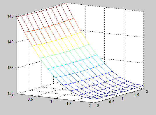
Problem 1: The primary elliptic partial differential equation upon which this assignment is based is u(xx) + u(yy) = (2*H/(K*delta))*u. This is solved using finite difference approximation using Robin Boundary conditions. We setup a 2x2 cm coolin fin with a width of 1mm (.1cm). 5 Watts of power were input on the left side, which was 2cm long. The connection represents a cpu giving off heat. The formula for the power to be input was P/(L*delta*K), which is (Power/((Length of Input)*(Width of input)*(Thermal Conductivity))). The graph using M = 10, N = 10 steps for the x, y directions is shown to the right. The maxiumum temperature found in the heat distribution was 144.9357 C, and the call to the p1() function listed below was p1(0, 2, 0, 2, 10, 10). Here's the Matlab code for this section.

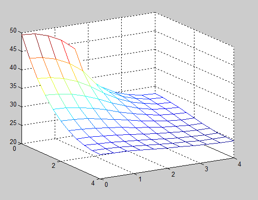
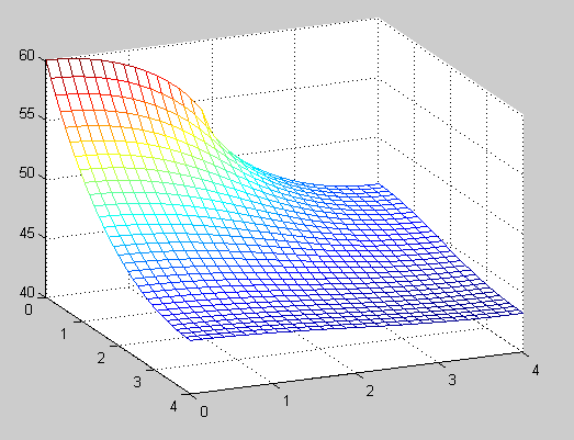
Problem 2: For this section, we increased the cooling fin to 4x4cm, while leaving the connection size at 2cm (the cpu is still the same size). Power is input along [0, 2], and the maximum temperature with 10x10 steps is 49.4704 C. When we increased the number of steps to 30x30 steps, the maximum temperature rose to 51.4560 C. The increased number of steps caused a higher max temperature to be calculated. Here's the Matlab code for this section.

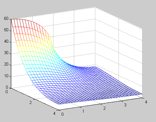
Problem 3: For this section of the project, the fin remained at 4x4 cm, the power input was still along 2cm, and we needed to calculate the maximum power wattage that could be input before the temperature rose above 80 C. The base bulk temperature was 20 C, and the Matlab code calculates temperature above the bulk temp, so we looked for temperatures below 60 C. When added to the bulk temperature, the total would be just under 80 C. We found that the power required to approach a maximum temperature of 60 C was 5.83 Watts. In finding this result, 30x30 steps were used. The p3() call used was p3(0, 4, 0, 4, 30, 30). Here's the Matlab code for this section.

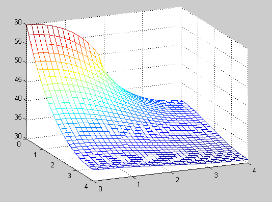
Problem 4: Next, we switched to a different material for the cooling fin. The new fin has a thermal conductivity of 3.85 W/(cm*C). The fin size is again 4x4 cm, and the connection with the cpu is 2 cm. As in the previous problem, we calculated the maximum number of Watts of power that could be input while maintaining a maximum temperature of below 80 C. The bulk temperature is still 20 C, so when the Matlab code gives a result of 59.9 C, it means 79.9 C in absolute terms. The power we determined for this limit was 7.40 Watts. We used 30x30 steps in order to get this result. The p4() call used was p4(0, 4, 0, 4, 30, 30). Here's the Matlab code for this section.

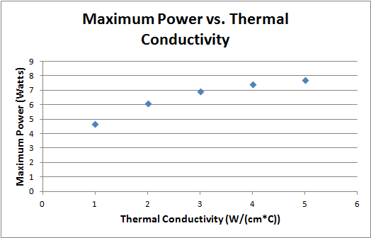
Problem 5: In this problem, we simply had to repeat problem 4 with thermal conductivity K going from 1 to 5. Then, we created a plot. The plot to the right shows the maximum power (with maximum temperature below 80 C) as a function of K, the thermal conductivity. The power values for K = 1, 2, 3, 4, 5 (W/(cm*C)) are (4.67, 6.1, 6.9, 7.4, 7.7) Watts. 30x30 steps were used in this calculation. Here, is the driver file for this problem, and here is the main function which performs finite differences.

Problem 6: Finally, we once again repeated problem 4 with all of the same conditions and constants except for H, the convective heat transfer coefficient. This was changed to 0.1 W/(cm^2*C) for a water cooled fin. The power we determined would reach just below 60 C above base boundary was 36.75 Watts. As usual, we used 30x30 steps. The Wattage for water with its higher convective heat transfer coefficient was much higher than for the other problems. Water is a highly effective means of removing heat. The call to p6() used was p6(0, 4, 0, 4, 30, 30). Here is the code for problem 6.