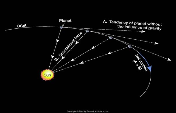
Introduction: For this project, we simulated the effects of gravity on various objects with different initial conditions. The magnitude of the gravitational force is G(m1)(m2)/(r^2). r is the distance between the two objects, G is a constant (6.67*10^(-11)). (However, in this project, G was set to the arbitrary value of 1). The gravity law indicates that the force of gravity becomes weaker with the square of the distance, and is directly proportional to the two masses multiplied together. The force acts along the unit vector pointing between them, and follows Newton's Third Law so that the second mass experiences a force opposite in direction and equal in magnitude to the first. For this project, the Runge Kutta Order 2 Method (Trapezoid) was used. When Euler's Method is used, it results in massive error, causing the orbit to spiral outward instead of forming an elliptical shape.

Two Body Problem: For this problem, mass 1 was set to 0.03, and mass 2 to 0.3. The initial conditions for mass 1 were (x: 2, y: 2), (vx: 0.2, xy: -0.2), and for mass 2 they were (x: 0, y: 0), (vx: -0.01, vy: 0.01). The video to the right shows that there is net system momentum, which drives the system to the lower right continually. Here's a table of the components of momentum for the individual masses, as well as the system as a whole.

p comp	mass 1	mass 2	system
x	0.03*0.2 = 0.006	0.3*(-0.01) = 0.003	0.006 + 0.003 = 0.009
y	0.03*-0.2 = -0.006	0.3*0.01 = 0.003	-0.006 + 0.003 = -0.003

The video plays at fairly slow speed for the first few moments, after which it is sped up in order to quickly display the way the system progresses over a longer period of time. This strategy is employed for the rest of the videos in this presentation as well. The matlab call orbit_two_body([0 100000], [2 0.2 2 -0.2 0 -0.01 0 0.01], 0.01, 5) was used to invoke the code shown below. Two Body Matlab m file

Three Body Problem (Stable): Three objects with precise intitial conditions are allowed to interact. Mass 1 was set to 0.03, mass 2 was set to 0.3, and mass 3 was 0.03. Here are the initial conditions:

Mass	Position	Velocity
m1	(2, 2)	(0.2, -0.2)
m2	(0, 0)	(0, 0)
m3	(-2, -2)	(-0.2, 0.2)

The code used to call the function was orbit_three_body([0 100000], [2 0.2 2 -0.2 0 0 0 0 -2 -0.2 -2 0.2], 0.01, 5). Three Body Matlab m file

Three Body Problem (Unstable): We also ran the same three body masses with one slight change in initial conditions for the x component of the starting velocity for mass 1. (went from 0.2 to 0.20001). This slight change causes the system to come flying apart, as can be seen in the video to the right. Here's the code used to invoke the function for this case with the slightly modified x velocity for mass 1. orbit_three_body([0 100000], [2 0.20001 2 -0.2 0 0 0 0 -2 -0.2 -2 0.2], 0.01, 5)

Figure 8 Orbit: This problem demonstrates a figure 8 orbit, and shows how it deteriorates as different values are added to the x velocity component for mass three. For this case, the masses were all set to 1, so they are all equivalent. This problem demonstrates even a small deviation from the initial conditions will destroy the system. Here's the code used to invoke the function for this case.

• figure8([0 1000000000], [-0.970 -0.466 0.243 -0.433 0.970 -0.466 -0.243 -0.433 0 0.932 0 0.866], 0.01, 5)
• Add 10^(-1) figure8([0 1000000000], [-0.970 -0.466 0.243 -0.433 0.970 -0.466 -0.243 -0.433 0 1.032 0 0.866], 0.01, 5)
• Add 10^(-2) figure8([0 1000000000], [-0.970 -0.466 0.243 -0.433 0.970 -0.466 -0.243 -0.433 0 0.942 0 0.866], 0.01, 5)
• Add 10^(-3) figure8([0 1000000000], [-0.970 -0.466 0.243 -0.433 0.970 -0.466 -0.243 -0.433 0 0.933 0 0.866], 0.01, 5)
• Add 10^(-4) figure8([0 1000000000], [-0.970 -0.466 0.243 -0.433 0.970 -0.466 -0.243 -0.433 0 0.9321 0 0.866], 0.01, 5)
• Add 10^(-5) figure8([0 1000000000], [-0.970 -0.466 0.243 -0.433 0.970 -0.466 -0.243 -0.433 0 0.93201 0 0.866], 0.01, 5)

Figure 8 (Add 10^-1): For this part of the figure 8 problem, 0.1 was added to the x-component of the starting velocity of mass three, taking it from 0.932 to 1.032. This results in a very rapid shift to the right of the figure 8 system, whereas the original remained stationary.

Figure 8 (Change by 10^-2): This time, 0.01 was added to vx for mass 3. The decay of the original state of the system takes longer than it did in the previous case in which 0.1 was added, but it still occurs quite noticeably and quickly.

Figure 8 (Change by 10^-3): We added 0.001 to mass 3's vx. This results in a slower shift to the right than for the previous cases.

Figure 8 (Change by 10^-4): 0.0001 was added this time, causing a very slow shift to the right. As can be seen in the accompanying accelerated video, the system slowly progresses in a rightward manner.

Figure 8 (Change by 10^-5): For the final case, 0.00001 was added to the initial x component of mass 3's velocity. The system shifts slightly to the right, taking even longer than all of the other cases. This 0.00001 addition is still enough to disturb the original system (hardly noticeable though). These figure 8 examples show the extreme reliance on initial conditions.