George Mason University

Zakaria Tarik Zerhouni

This project was completed in collaboration with Harout Boujakjian and Elisa Kim

Website designed by Conor P. Nelson

Project 3: Differential Equations Modeling

The goal of this project is to model by means of a system of differential equations the motion of a pendulum under gravity.

In order to accomplish this we will first define our coordinate system.

It is assumed that the pendulum is hanging from a rigid rod, and is free to pivot 360 degrees. The pendulum will be under the force of gravity and the downward position at 6 o'clock will be the angle \( 2k \pi \), where \( k \in \mathbb Z \).

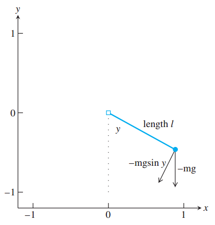
We will take \(y\) to be the anglular displacement of the pendulum from 6 o'clock.

The length of the pendulum rod will be \( l \) and this will constrain the bob of the pendulum to a circle of radius \( l \). Our positional component will then be the arc length \( s = r \theta \), which will be \( ly \).

The component of acceleration tangent to the circle is then \( ly'' \). As the component of force along the direction of motion (as a restoring force) is \( F = -mg \sin y \), and taking into consideration Newton's second law of motion, commonly formulated as \( F = ma\), it becomes clear that

\( \displaystyle ly'' = a = -g \sin y \). (Equation 0.1)

Figure 0.1

Figure 0.1 sketches the positions and forces detailed above.
Taken from Numerical Analysis: Second Edition authored by Timothy Sauer.

This will be the differential equation used to model our pendulum. However, as it is a second-order differential equation, we will redefine the equation as a system of differential equations where \( y_1 = y \) and \( y_2 = y' \). Note that \(y_2' = y''\).

Thus we have the system of differential equations modeling our pendulum under gravity as,

System 0.1

\( \displaystyle y_1' = y_2 \),
\( \displaystyle y_2' = - \frac{g}{l} \sin y_1 \).

By using the trapezoid method of approximating the solution of a system of differential equations, we were able to create a MatLab program animating our pendulum.

System 0.1 models only simple harmonic motion. In each stage of our investigation we will experiment with and analyse our pendulum under different conditions.

We will introduce forcing and damping into the model and then we will proceed to introduce an oscillating pivot in order to stabilize our pendulum when inverted. As a final challenge, we will model a double pendulum and then attempt to stabilize it.

Our results are presented in the steps tabulated below.

Project 3: Chapter 6 Computer Simulation: The Pendulum

Step 1: Build a forced, damped animation of a pendulum.

Step 2: Multiple attracting trajectories and chaotic motion.

Step 3: The oscillating pivot and parametric resonance.

Step 4: More on parametric resonance.

Step 5: The double pendulum.