|
|
George Mason UniversityZakaria Tarik ZerhouniSource: Home > Project 4 > Part 2Math 447: Numerical Analysis
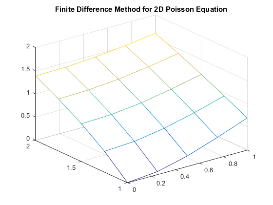
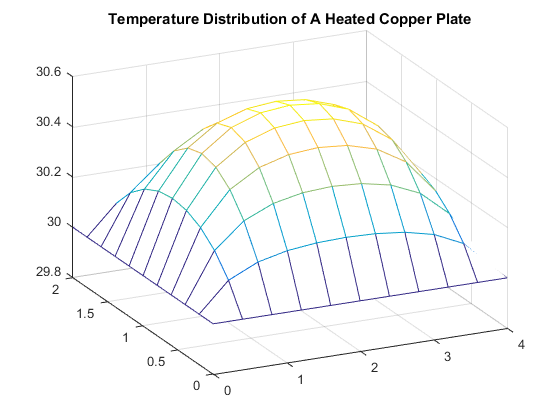
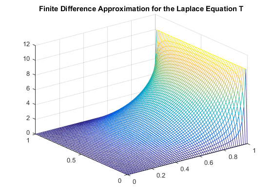
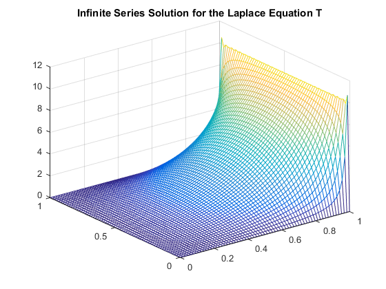
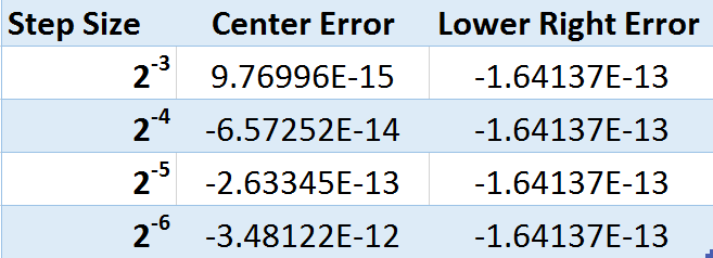
The Laplace equation we address deals with the Laplace of a twice differentiable function \( u(x, y) \) whose Laplacian meets the conditions \( \Delta u(x, y) = 0 \). In order to master the skills required to solve for solutions of this form using the Finite Difference Method, we solved for the simple example of \( \Delta u = 0\) on the interval \( [0, 1]_x \times [1, 2]_y \) with the Dirichlet boundary conditions \( \left\{ \begin{array}{lr} u(x, 1) = \ln(x^2 + 1) \\ u(x, 2) = \ln(x^2 + 4) \\ u(0, y) = 2\ln(y) \\ u(1, y) = \ln(y^2 + 1) \end{array} \right.\) We went on to model the steady-state temperature \(u\) on a heated copper plate, which meets the conditions of a Poisson equation as \( \Delta u = -\frac{D(x, y)}{K} \) where the power density \(D(x, y) \) will be \( D(x, y) = 5 \frac{watts}{{cm}^3} \) and the thermal conductivity of copper \(K\) is \( K = 3.85 \frac{watts}{{cm}^\circ C} \) on the interval (in centimeters) \( [0, 4]_x \times [0, 2]_y \) and keeping the temperature at the boundaries at a constant \({30}^\circ C\) with the Dirichlet boundary conditions \( \left\{ \begin{array}{lr} u(x, 0) = 30 \\ u(x, 2) = 30 \\ u(0, y) = 30 \\ u(4, y) = 30 \end{array} \right.\) From our Finite Difference Approximation of the heat distribution we found that that temperature at the center of the plate \((x, y) = (2, 1)\) was: \( 30.587882974920344 \). The next investigation addressed the Laplace equation \( \Delta T (x, y) = 0 \) on the interval \( [0, L]_x \times [0, H]_y \). For this Laplace equation the Dirichlet boundary conditions are defined as, \( \left\{ \begin{array}{lr} T(x, 0) = T_0 \\ T(x, L) = T_0 \\ T(0, y) = T_0 \\ T(H, y) = T_1 \end{array} \right.\) We were able to show that for, \(C_k = \frac{4(T_1 - T_0)}{(2k+1)\pi \sinh \frac{(2k+1)\pi H}{L}}\), and, \( T(x, y) = T_0 + \sum\limits_{k=0}^n C_k \sin \frac{(2k+1)\pi x}{L} \sinh \frac{(2k+1)\pi y}{L}\), we have a solution to \( \Delta T = T_{xx} + T_{yy} \). Note that \( C_k \) is a constant value in each element of the summation. \( T(x, y)_{xx} = \sum\limits_{k=0}^n -C_k \frac{(2k+1)^2\pi^2}{L^2} \sin \frac{(2k+1)\pi x}{L} \sinh \frac{(2k+1)\pi y}{L}\) \( T(x, y)_{yy} = \sum\limits_{k=0}^n C_k \frac{(2k+1)^2\pi^2}{L^2} \sin \frac{(2k+1)\pi x}{L} \sinh \frac{(2k+1)\pi y}{L}\) As each element in \(T_{xx}\) for every \(k\) is the negative of the same element for that \(k\) in \(T_{yy}\) we have, \(T_{xx} +T_{yy} = \sum\limits_{k=0}^n -C_k \frac{(2k+1)^2\pi^2}{L^2} \sin \frac{(2k+1)\pi x}{L} \sinh \frac{(2k+1)\pi y}{L} + \sum\limits_{k=0}^n C_k \frac{(2k+1)^2\pi^2}{L^2} \sin \frac{(2k+1)\pi x}{L} \sinh \frac{(2k+1)\pi y}{L}\). And so, \(\Delta T = T_{xx} +T_{yy} = 0 \). We went on to solve \(\Delta T\) with a finite difference approximation on \( [0,1]_x \times [0,1]_y \), for \(T_0 = 0\) and \(T_1 = 10\). To check that the correct plot was produced the solution in the form of an infinite series was computed with a hundred steps of the summation. As can be seen below, there are no significant visually discernible differences. To check the error of the approximate solution against the infinite series, the four points at the corners of the plot and the center of the plot were tested. There was no difference in the computation value for the upper left, upper right, and lower left points of the plot. The error stayed the same of each step size at the lower left point. However, surprisingly, the error in the center grew as the step size became smaller. This may be due to the fact that the infinite series, only computed for 100 steps, could not converge close enough to the solution against the approximate value for the associated step size. Table 1: Error
|
