Introduction to Connected Components and the Project

What it means to be connected

Spectral clustering is a method of clustering data that relies on eigenvalues to clump data into sets. We, naturally, have an inutition for what it means for a set of objects to be clustered. Our visual processing has evolved to search for patterns and separate sets of data. However, there is no universal, intuitive algorithm for data sorting. In spectral clustering, a similarity matrix is first defined. A similarity matrix A has the property that \(a_{ij}\) contains information regarding how ``similar'' points \(i\) and \(j\) are. From this matrix, what is known as a Laplacian matrix is constructed. A Laplacian matrix is a matrix representation of a graph. Wikipedia gives an excellent example of a graph, its degree matrix, its adjacency matrix (similarity matrix), and its Laplacian matrix. The eigenvectors and eigenvalues for this Lapalcian matrix are then found. Partitioning of the points is then performed based on the eigenvectors and values.

An example method of partitioning is as follows: consider the second-smallest eigenvalue of the Laplacian matrix and its corresponding eigenvector; for all points with a component in said eigenvector less than the value of the eigenvalue, place the points in one set; then place all other points in a separate set; additional partitions may be applied on this next set with respect to the next eigenvalue. There are many methods of spectral clustering, but this is simply one example. The graph Laplacians used throughout this project differ, and are each covered in turn.

The Project

We begin with a union of connected components in \(\mathbb{R}^n\) and fix an \(\epsilon > 0\). Then our initial weight matrix \(W\) is defined as \(W_{ij} = 1 \text{ if } ||x_i - x_j|| \lt \epsilon\) and 0 otherwise for all paris of points \(x_i,\,x_j\) and implemented in ndimweightmatrix.m. We also occasionally use an alternate weight matrix that is defined as \(W_{ij} = \text{exp}(-\frac{||x_i-x_j||^2}{2\epsilon^2})\). Then \(D\) is defined as the diagonal matrix of the row sums of \(W\).

Then we have our choice of a graph Laplacian from the following list:

1. Unnormalized: \(L = D - W\)
2. Symmetric: \(L_{\text{sym}} = I - D^{-0.5} W D^{-0.5}\)
3. Random Walk: \(L_{\text{rw}} = I - D^{-1}W\)

Using MATLAB's [V, D] = eig( A ) command we may find the eigenvalues and corresponding right eigenvectors of our chosen Lapalcian. Our graph Laplacian is symmetric with nonegative eigenvalues and the eigenspace corresponding to \(\lambda = 0\) is spanned by the vectors \(D^{0.5}\textbf{1}_{S_i}\), where \(\textbf{1}_{S_i}\) is an indicator function. Since the eig command returns some orthogonal basis for the eigenspace, we must "unmix" the eigenvectors to obtain the appropriate indicator functions.

In order to unmix the eigenvectors, we let \(E\) be the \(N \times c\) matrix of eigenvectors returned where \(N\) is the number of data points and \(c\) is the number of clusters. We then apply the \(PA=LU\) factorization to \(E\) and define \(M\) as the \(N \times c\) matrix formed by the top \(c\) rows ot \(PE\). Then the columns of \(EM^{-1}\) serve as the indicator functions for the clusters. A MATLAB implementation is as follows:

Disks in the Plane

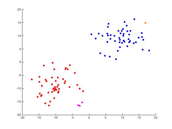
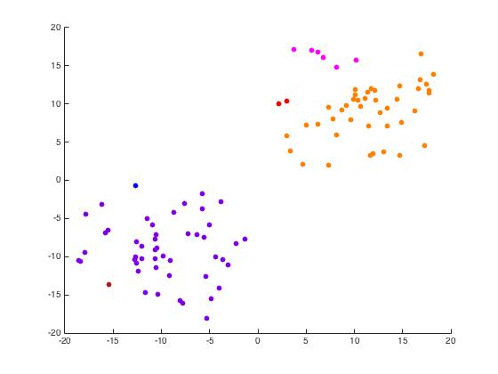
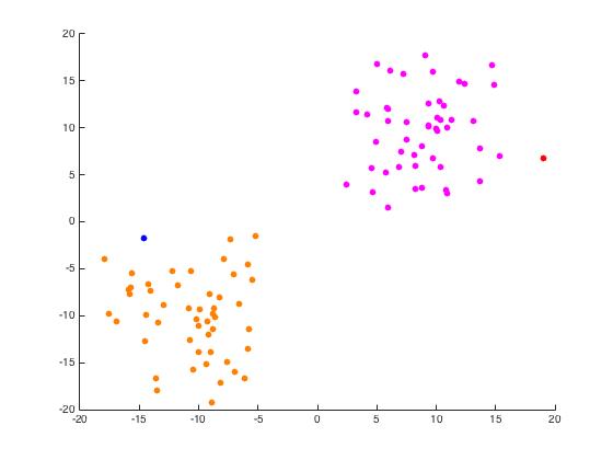
For this part of the project, we begin with a random set of points in \(\mathbb{R}^2\) arranged in two distinct disks generated by randomdiskpoint.m. We then used projectmain.m to generate the following plots. It is important to note that this code does not attempt to unmix the eigenvectors as the project description states we should.

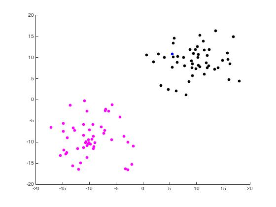
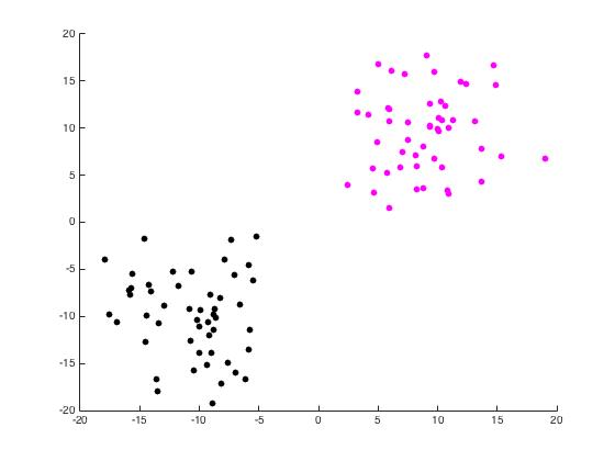
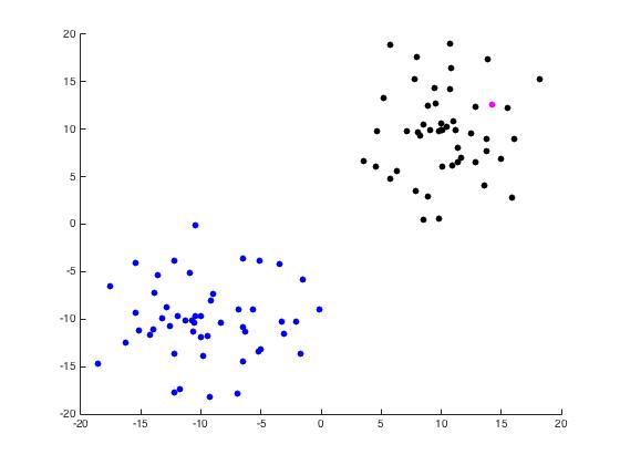
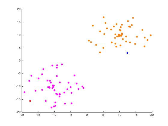
Now we use unmixing_code.m to perform the same task while unmixing the eigenvectors as the name would suggest.

Iris Data Set

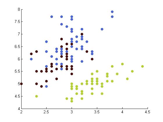
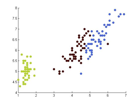
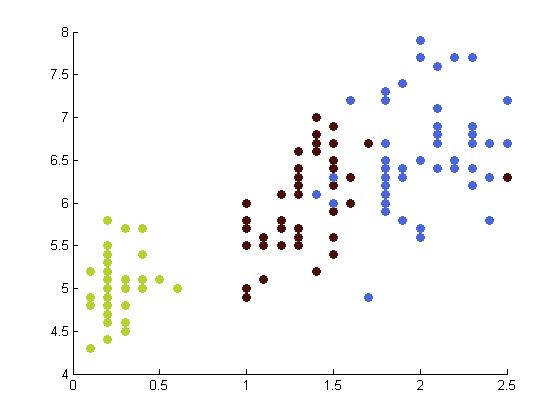
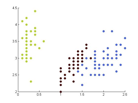
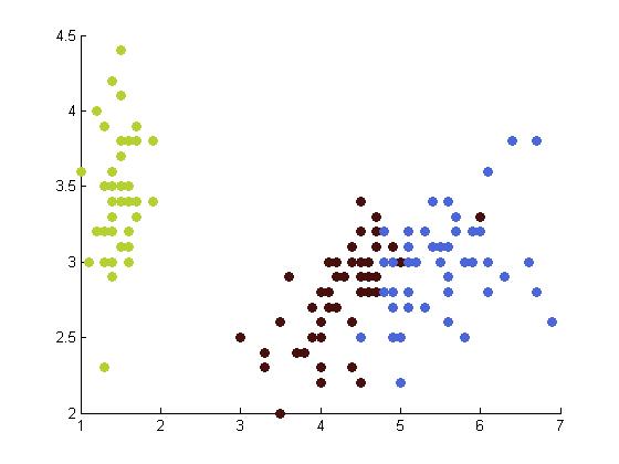
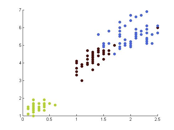
The following table depicts the clustering results for the Iris dataset and are arranged to correspond to the image on the Wikipedia page. The images were produced by projectmainIris.m. Again note that this file does not unmix the eigenvectors.

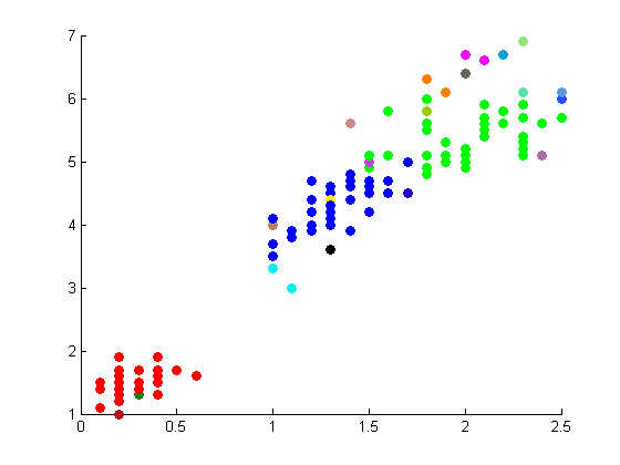
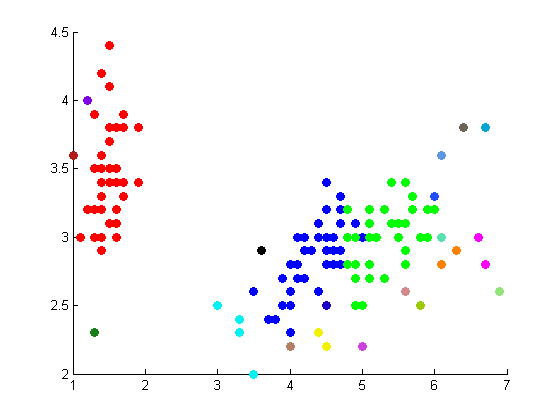
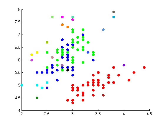
The following figures depict the results from projectmainIris(Daniel). This code makes use of the random walk graph lapalcian, standard weight matrix, and eigenvector unmixing.

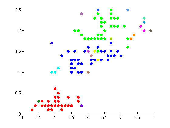These results are not as well correlated with the correct clustering shown on the Wikipedia page.

A Ring

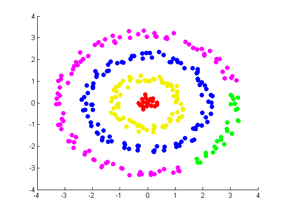
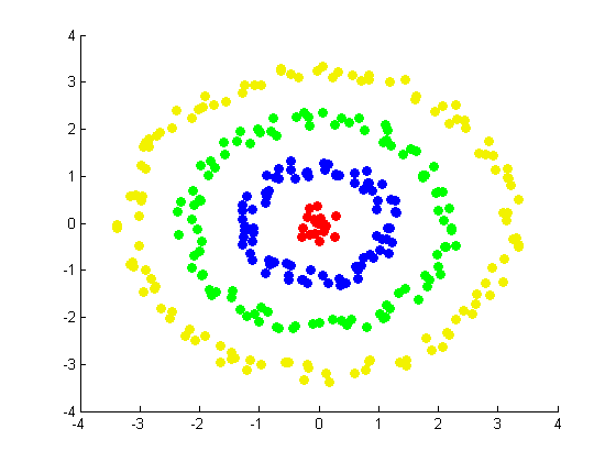
Our next and final exhibit (constructed by Daniel) involves a set of random points arranged in a target pattern. Using ringdataset.m and projectmainRing.m, which make use of the random walk graph Laplacian and the alternative weight matrix constructed in ndimALTweightmatrix.m, we constructed the follwoing figures: