Heats travels from the hot spot to the cooler spots. We were to make heat enter at one end of a fin and make sure that the temperature of the fin would stay within a safe tolerance. The fin that we were to make was a rectangular fin with Lx \(\times\) Ly with a width of \(\delta\) cm, keeping in mind that \(\delta\) is relatively small. Since our \(\delta\) is so small we use the function u(x,y) where \(\delta\) is a constant that is included with the Ly.
Heat moves in three ways: conduction, convection and radiation. Let's examine each in the following paragraphs.
Conduction: the passing of energy between neighboring molecules. Conduction follows Fourier's first law and we used the following equation:
We define q as the heat energy per unit time, which is measured in watts. We define A as the cross-sectional area of the material. We define \(\nabla\)u as the gradient of the temperature. Our constant K is the Thermal Conductivity of the material.
Convection: the passing of energy between neighboring molecules due to the movement of electrons. Convection follows Newton's law of cooling and we used the following equation:
Variables that were previously defined stay the same. But the new variables are as follows, H, and ub. We define H as the proportionality constant called the convection heat transfer coefficient. We define ub is the ambient temperature of bulk temperature of the fluid surrounding the object. In our case the fluid surrounding the fin is air.
Radiation: the movement of energy through photons. But for the sake of this project we will not worry about it.
In our code we were to define our boundaries of our [0,Lx] \(\times\) [0,Ly] \(\times\) \(\delta\) cm. Energy equilibrium in a typical fin means that energy entering the fin equals the energy exiting the fin. The heat entering is called the heat flux, via conduction and gives us the equations:
In this particular example ub = 0, which means that the rest of the time u will be the difference between the fin and its surrounding. When we divide by \(\Delta\)x\(\Delta\)y and take the \(\lim_{\Delta x\rightarrow0}\)and \(\lim_{\Delta y\rightarrow0}\), then we get the following equation:
We have a similar argument that implies convective boundary condition or a Robin boundary condition.
unormal is a partial derivative with respect to the outward normal direction \(\vec n\). In this project we are assuming that the power enters along one side of the fin thus Fourier's law allows us to use this next equation:
Where P is the total power and L is the length of the input.
To find the interior points (xi,yj) where 1\(\lt\) i\(\lt\)m and 1\(\lt\) j\(\lt\)n, for integers m and n. And follows the following equation:
f'(x) = \(\frac{-3f(x)+4f(x+h)-f(x+2h)}{2h}\)+O(h2)
We must also find the values at the edges of the fin, to do so we need the following equations, the last part of the equations are the second-order first derivative approximation:
Top Edge: unormal = uy \(\approx\) \(\frac{-3u(x,y)+4u(x,y-k)-u(x,y-2k)}{-2k}\)
Left Edge: unormal = -ux \(\approx\) \(\frac{-3u(x,y)+4u(x+h,y)-u(x+2h,y)}{2h}\)
Right Edge: unormal = ux \(\approx\) \(\frac{-3u(x,y)+4u(x-h,y)-u(x-2h,y)}{2h}\)
And if we combine the last equation of each of the above equations with the Robin boundary condition leads to the following equations:
Top Edge: \(\frac{-3u_{in}+4u_{i,n-1}-u_{i,n-2}}{2k}\) = -\(\frac{H}{K}\)uin
Left Edge: \(\frac{-3u_{1j}+4u_{2j}-u_{3j}}{2h}\) = -\(\frac{H}{K}\)u1j
Right Edge: \(\frac{-3u_{mj}+4u_{m-1,j}-u_{m-2,j}}{2h}\) = -\(\frac{H}{K}\)umj
In this project we are assuming that the power enters along the left side of the fin thus Fourier's law allows us to this next equation:
We are solving mn equations and mn unknowns.
For the purposes of this project, we were to assume that K = 1.68 \(\frac{W}{cm ^\circ C}\), H = 0.005 \(\frac{W}{(cm^2)^\circ C }\) and ub = 20 \(\circ\)C
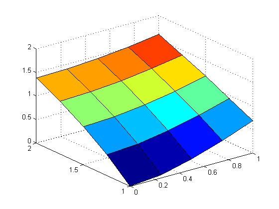
We needed to make code that worked, here is the graph that matches what is in the book meaning that our coding worked.
All we needed to do was go to the course website and download the poisson.m file and then run the code and we got the following image:

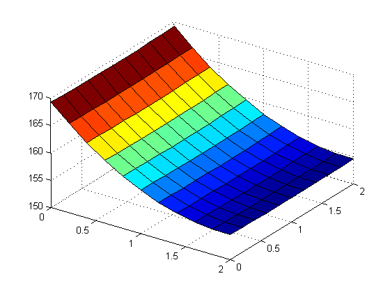
For this part of the project we began with a fin with the dimensions of 2 \(\times\) 2 cm and 1 mm thickness. We assumed that 5W of power was the input along the left edge of the fin, as if the fin were attached to dissipate power from a CPU chip with L = 2 cm side length. We were to solve the PDE with M = N = 10 steps in the x and y directions. We were also to solve the maximum temperature of the fin in \(\circ\)C.
\(\star\)\(\star\) NOTE: For the entire project instead of using the mesh command as suggested in the book we used the surf command which gave us a better image to look at, and would look better from the projector.\(\star\)\(\star\)
\(\star\)\(\star\)ALSO NOTE: Our axes are not labelled so that we can have a better view of the graph. The x and y axes are on the left and right while the z axis is going up. Where the x and y axes are the dimensions of the fin and the z axis is the temperature.\(\star\)\(\star\)
Below is the graph that we got after running the program and when you click on if you can see that code that we used to create the graph.
For this part of the project we increased the dimensions of the fin with to 4 \(\times\) 4 cm and 1 mm thickness. We assumed that 5W of power on the interval [0,2] on the left side of the fin. We were to solve the PDE with M = N = 20 steps in the x and y directions. We were also to solve the maximum temperature of the fin in \(\circ\)C. And finally we were to experiment with increased values of M and N and to see how much the solution was to change.
Below is the graph that we got after running the program and when you click on if you can see that code that we used to create the graph. The different M=N sizes are as follows for the following figures respectively: N=M=15, N=M=30, N=M=100.
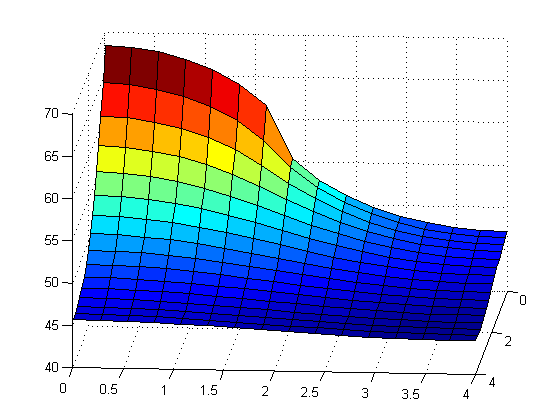
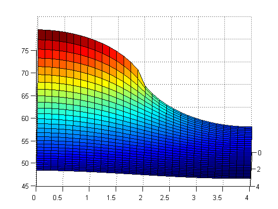
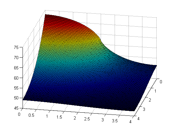
It can be seen that as N and M increase where the color changes becomes more defined and exact. But for the most part the colors are staying the same in their places.
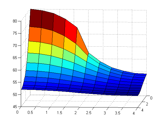
For this part of the project we were to find the maximum power that was dissipated by the 4 \(\times\) 4 cm fin while keeping the maximum temperature less than 80\(\circ\)C. We were to assume that the bulk temperature was 20\(\circ\)C and the power input along 2 cm.
Below is the graph that we got after running the program and when you click on if you can see that code that we used to create the graph.
Bisectionmethod.m was used to find the maximum power that could be dissipated on a 4 \(\times\) 4 cm fin with the 2 cm power input. We did not define this function ended up giving us the value 6.006543165477551 for the maximum amount of power.
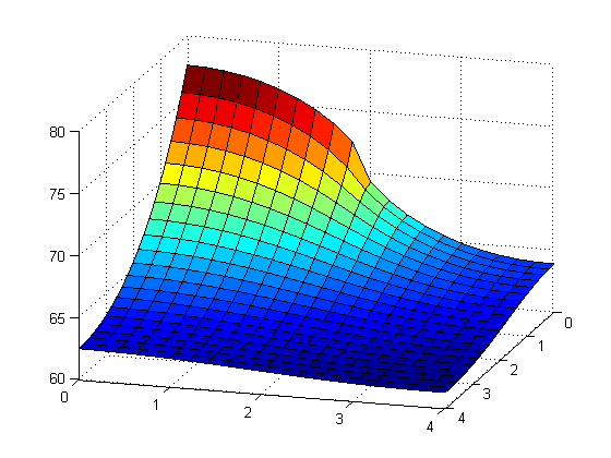
For this part of the project we were to use a copper fin instead of an aluminum fin. The copper fin has K = 3.85\(\frac{W}{cm ^\circ C}\). We were to again find the maximum power that could be dissipated by 4 x 4 cm with the 2 cm power input in the optimal placement, while keeping the maximum temperature below 80\(\circ\)C.
Bisectionmethodcop.m was used to find the maximum power that could be dissipated on a 4 \(\times\) 4 cm fin with the 2 cm power input. This function ended up giving us the value 7.136096462619060 for the maximum amount of power.
Below is the graph that we got after running the program and when you click on if you can see that code that we used to create the graph.
We were to plot the maximum power that can be dissipated in the previous problem. We had the function to be for 1\(\le\)K\(\le\)5\(\frac{W}{cm ^\circ C}\)
Below is the graph that we got after running the program and when you click on if you can see that code that we used to create the graph.

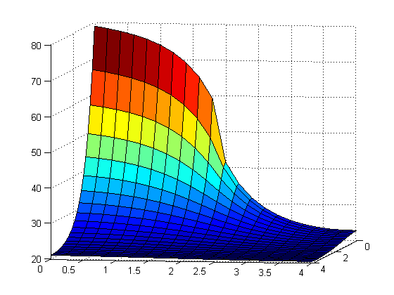
For this part of the project we were to do the same steps as in step 4 but with a water-cooled fin. We assumed that water has a convective heat transfer coefficient of H = 0.1 \(\frac{W}{(cm^2)^\circ C }\) and that the ambient water temperature is maintained at 20\(\circ\)C.
Bisectionmethod6.m was used to find the maximum power that could be dissipated on a 4 \(\times\) 4 cm fin with the 2 cm power input. This function ended up giving us the value 20.555273672122084 for the maximum amount of power.
Below is the graph that we got after running the program and when you click on if you can see that code that we used to create the graph.
Instead of doing as suggested in the book for problem 7, we did something different. We had two or three places where we would have heat entering the fin.
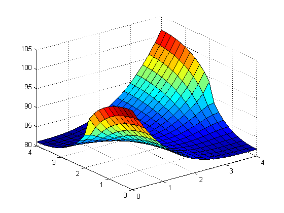
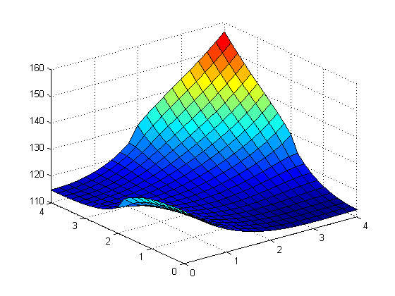
In the first image above we had heat entering the cooling fin from \([0,2]\) on the left side and \([2,4]\) on the right side. In the second image we had power from \(y=[0,2]\) on the left side and \(y=[2,4]\) on the right side and also from \(x=[2,4]\) on the top side.
It was interesting to see how the different step sizes could affect the boundaries of the cooling fin. The most interesting part of this project was the having heat enter the fin at many points.
Coding completed in class: mainly Theo and Peter
Webpage constructed by Chelsea
