This project explores the mathematics behind the global positioning system (GPS), a network which consists of 24 satellites carrying atomic clocks that orbit the earth at an altitutude of 20,200 km. Each satellite has a simple mission: to transmit carefully synchronized signals from predetermined positions in space to be picked up by GPS receivers on earth. The receivers use the data to calculate accurate \(x, y, z\) coordinates of the receiver and determine the transmission time.
We employed the Multivariate Newton's Method to solve for the receiver position \((x, y, z, d)\) near earth and time correction \(d\) using 4 satellites with known positions.
We first begin by examining the case of 4 satellites with \((A, B, C)\) coordinates that were given as part of the problem:
| Satellite (\(n\)) | \(A_i\) \(x\)-position | \(B_i\) \(y\)-position | \(C_i\) \(z\)-position | transmission time \(t_i\) |
|---|---|---|---|---|
| 1 | 15600 | 7540 | 20140 | 0.07074 |
| 2 | 18760 | 2750 | 18610 | 0.07220 |
| 3 | 17610 | 14630 | 13480 | 0.07690 |
| 4 | 19170 | 610 | 18390 | 0.07242 |
The system of equations given with the project were algebraically manipulated into the form of below.
\begin{align*} f_1 = (x - A_1)^2 + (y - B_1)^2 + (z - C_1)^2 - (c(t_1 - d))^2 = 0\\ f_2 = (x - A_2)^2 + (y - B_2)^2 + (z - C_2)^2 - (c(t_2 - d))^2 = 0\\ f_3 = (x - A_3)^2 + (y - B_3)^2 + (z - C_3)^2 - (c(t_3 - d))^2 = 0\\ f_4 = (x - A_4)^2 + (y - B_4)^2 + (z - C_4)^2 - (c(t_4 - d))^2 = 0 \end{align*}
Thus we want to solve the system of equations for \(i = \{1,2,3,4\}\) using a multivariate Newton's to be sure that our \((x,y,z,d) = (-41.77271, -16.78919, 6370.0596, -.003201566)\). Attached here is our MATLAB code, and below is an example run of this code. Newton's method took 4 iterations to converge to the answer with an initial guess of (0, 100, 6400, 0.0001).
We are solving the same system of equations as in Part 1, except this time we will use the Quadratic Formula. We are doing so by subtracting the last 3 equations from the first, which yields 3 linear equations in the four unknowns \(u=(x,y,z,d\)), or in Matrix from \( Au = b\) in a 3 by 4 matrix.
The MATLAB code for Step 2 .
The results of Step 2 can be viewed here.
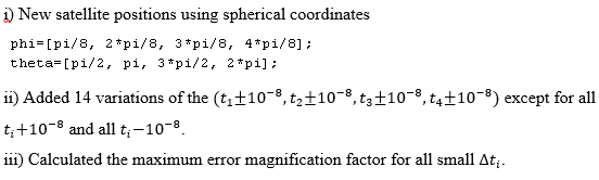
Set up new satellite locations using spherical coordinates, and find the maximum error magnification factor for all small \(\Delta t_i=10^{-8}\).
Define satellire positions \((A_{i},B_i, C_i)\) from spherical coordinates \((\rho, \theta, \phi)\) as:
\(\begin{align*} A_i &= \rho\cos\phi_{i}\cos\phi_{i}\\ B_i &= \rho\cos\phi_{i}\sin\phi_i\\ C_{i}&= \rho\sin\theta_i \end{align*}\)
where \(\rho = 26570\) km and \(\phi\) values are arbritrarely chosen between \([0, \frac{\pi}{2}]\), \(\theta\) between \(\left[0,2\pi\right]\), for \(i = \{1,2,3,4\}\).
Set \((x,y,z,d) = (0,0, 6370,0.0001)\), and calculate the corresponding ranges \(R_i\) and travel time \(t_i\):
\(\begin{align*} R_i &= \sqrt{ A_i^2 + B_i^2 + ( C_i - 6370)^2 }\\, t_i &= d + R_i / c \end{align*}\)
\(\begin{equation*} EMF = \frac{||(\Delta x, \Delta y, \Delta z)||_{\infty}}{c||\Delta t_{i}||_{\infty}} \end{equation*}\)
Followings are changed from Step 1 code.
The maximum error magnification factor for all small \(\Delta t_i\) (condition number)
= 5.475302028519095.
Repeat Step 4 with a more tightly grouped set of satellites.
From Step 4, choose all \(\phi_i\) and \(\theta_i\) within 5 percent of one another.
Only spherical coordinates of satellite positions were changed from Step 4 code.
\(\begin{align*} \phi &= \left[ \frac{ \pi}{8} + \frac{0.01 \pi}{2}, \frac{\pi}{8} + \frac{ 0.02 \pi}{2} ,\frac{ \pi}{8} + \frac{0.03 \pi}{2}, \frac{\pi}{8} + \frac{0.04 \pi}{2}\right]\\ \theta &= \left[ \frac{\pi}{2} + (0.01)(2 \pi), \frac{\pi}{2} + (0.02)(2 \pi) , \frac{\pi}{2} + (0.03)(2 \pi), \frac{\pi}{2} + (0.04)(2 \pi) \right] \end{align*}\)
The maximum error magnification factor for all small \(\Delta t_i\) (condition number)
= 1.083912067236088e+05.
These tightly bunched satellites show larger condition number than the loosely bunched satellites in Step 4.
That is, tightly bunched satellites are less accurate than unbunched satellites.
Decide whether the GPS error and condition number can be reduced by adding satellites.
Return to Step 4, and add three more satellites. Now assume that we know locations of seven satellites.
Followings are changed from Step 4 code.
i) Seven satellite positions
\(\begin{align*} \phi &= \left[ \frac{2 \pi}{16}, \frac{3 \pi}{16} ,\frac{4 \pi}{16}, \frac{5 \pi}{16}, \frac{6 \pi}{16}, \frac{7 \pi}{16} , \frac{8 \pi}{16}\right]\\ \theta &= \left[ \frac{2 \pi}{4}, \frac{3 \pi}{4} ,\frac{4 \pi}{4}, \frac{5 \pi}{4}, \frac{6 \pi}{4}, \frac{7 \pi}{4} , 2 \pi \right] \end{align*}\)
ii) Random 14 variations of the \(\Delta t_i±10^-8, i=1,..,7\) though possible combination is \(2^7\).
iii) Used Gauss-Newton iteration to solve the least squares system of seven equations in four variables (x, y, z, d).
The maximum error magnification factor for small \(\Delta t_i\) (condition number)
| Step 4 - 4 Satellites | Step 5 - 4 Satellites | Step 6 - 7 Satellites |
|---|---|---|
| 5.475302028519085 | 1.083912067236088 e^05 | 6.587842923414091 |
The bunched satellites are less accurate than unbunched satellites.
Adding more satellites does not provide more accurate position.