


In my last post about March Madness, I talked about scraping and refining data for all 12,122 NCAA women’s and men’s Division I basketball games down to nice little summaries for each team in the tournament. To recap, the experimental setup is this:
- Compile a database of boxscores for all of this season’s NCAA Division I men’s and women’s college basketball games.
- Compile a database of NET rankings for the same.
- Put the databases from (1) and (2) together to make a giant database of every single game with specific statistics attached.
- For each team in the Tournament:
- look in the database from (3) for all the games the team has played;
- find “signal” games to tell us how that team does against certain types of teams (better, worse, just-as-good) and in certain types of games (close games, conference games, neutral-court games);
- assign each of these “signal” games a score (that I call the ) based on some (weighted) combination of statistics;
- create a fact sheet for the team for quick-referencing the different types of teams, games, and s.
- Make brackets. That means individually assessing each matchup and sometimes taking guesses. Hopefully, with all this data in our back pocket, those guesses will be educated ones.
- Post-Tournament post-mortem to assess how this year’s version of the did.
I’m on to Step 4.2, where I scrounge for a scrap of signal in a sea of noise.
Deciding which game types to include in a measurement of a team’s upset potential is hard. Sometimes, variables confound: do close games indicate a team’s ability to close out, or do they suggest a team is weak to lower-ranked competition? If a team mostly plays against worse competition, what happens when they run into better? When do the NET and AP rankings accurately reflect team strength? Does NCAA Tournament seeding even matter? All excellent questions, none answerable by me. I have a rough, uneducated philosophy, though, so let’s work from there.
To me, volatile teams are prone to upsets, whether those upsets are wins or losses. A “volatile” team is one that regularly loses games they should win, or wins games they should lose. The University of Virginia Cavaliers are a great example of a volatile team entering this year’s tournament. Between January 1st and Selection Sunday, the Hoos hovered between 36th and 39th in the NET and had these results:
- narrowly beat Florida State (109) and Georgia Tech (94);
- lost to Virginia Tech (41) twice, Syracuse (41) once, California (51) once, and split games with Clemson (42);
- beat Louisville (12), Notre Dame (36), and nearly knocked off NC State (12).
It seems like UVA is equally capable of winning and losing games they shouldn’t. The Hoos were dubbed a 10-seed in the Tournament despite an end-of-season NET ranking of 36 and, in the Tournament, upset 7-seed Georgia and 2-seed Iowa in Iowa City, then put up a good fight against 3-seed TCU. (If I recall correctly, UVA’s upset against Iowa busted every remaining women’s bracket on ESPN’s bracket challenge.) Georgia was only ranked 34th in the end-of-season NET, and had upset wins against Ole Miss (19), Kentucky (13), and Vanderbilt (7) under their belt. The Georgia–UVA game went to overtime — and the Iowa–UVA game to double overtime — but UVA prevailed in duplicate. How am I supposed to decide whether a team leans more towards upsetting or being upset?
I don’t. I just make separate “will-upset” and “be-upset” s, then compare.
If I’m building two scoring methodologies — bearing in mind that I am lazy — I’m going to build them in basically the same way and not go too crazy. My questions now are thus:
What subsets of games are important for diagnosing upset potential?
To me, past is prologue. Want to decide whether a team’s gonna get upset? Look at how they performed against worse and about-as-good teams, in upset losses, and in near-misses. Want to decide whether a team’s going to upset someone else? Check how they did against better teams, in away games, and in close games they won. More precisely:
| will-upset | be-upset |
|---|---|
| Upset wins (duh) | Upset losses (equally duh) |
| Close games against better teams | Close games lost against worse teams |
| Wins against teams close in the NET | Losses against teams close in the NET |
| Near-misses |
Each of these game types are weighted equally. Since near-miss games can show up in both columns, sometimes a game can count both for and against you. (This is an unfortunate side effect that comes from sample size: sometimes, teams just don’t play enough games to get an accurate picture of their opposition-agnostic performance, and I’m forced to double-count games. Oh well.)
What data do I consider, and how do they stack up against each other?
I restrict myself to three qualitative variables (win/loss, conference/nonconference, home/neutral/away) and three real-valued ones (focus/opponent NET strength, days since the game). For (e.g.) the will-upset , I look at all the games in the will-upset column above, apply the transformations below to the variables, multiply the outcomes to get s, then sum the s across all will-upset games.
Here’s how I treat the qualitative variables:
| Variable | Schema |
|---|---|
| Win/Loss | For the will-upset , a won game contributes \(1\) point and a lost game contributes \(\nicefrac 78\)ths of a point. For the be-upset , flip these. |
| Conference | Conference games contribute \(1\) point and non-conference games \(\nicefrac 34\)ths of a point. |
| Location | A neutral-site game always contributes \(\nicefrac {15}{16}\)ths of a point. For the will-upset , an away game contributes \(1\) point and a home game \(\nicefrac 78\)ths; flip these for the be-upset . |
Each of the real-valued variables are transformed by a logistic function \[\mathcal L_\gamma(x,y) = \frac{1}{1 + e^{\gamma(x-y)}}, \] where \(\gamma\) controls the slope of the curve and \(y\) is the coordinate of the axis of symmetry. Here’s the logistic function \(\mathcal L_{\nicefrac{1}{16}}(x, 70)\) that specifies the weight of a game according to the number of days \(x\) since it was played:
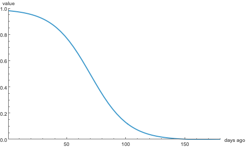
The logistic function \(\mathcal L_{\nicefrac{1}{16}}(x, 70)\).
Plainly, the predictive value of a game decreases with time; at first gradually, then exponentially quickly, then gradually again, losing half its value in 70 days. Logistic functions of this form always take values between \(0\) and \(1\), so each of our scores will be bounded by the same. Here’s how I transform the real-value variables:
| Variable | Schema |
|---|---|
| Strength | Let \(I\) be the in-focus team’s NET ranking and \(O\) the opponent’s. For the will-upset , I use \(\mathcal L_{\nicefrac 14}(O, 25)\); this means that an upset win’s value is based entirely on the opponent’s strength. I do this to numerically filter out games that are technically upsets (like the 245th NET team beating the 230th) but aren’t really. And, since the goal is to beat the best teams in the country, this rule forces teams to demonstrate they can do so. For the be-upset , it’s \(\mathcal L_{-\nicefrac 14}(O, I+15)\). Transforming this way has the effect of attenuating the worth of an upset loss according to the in-focus team’s strength: if South Carolina (NET 3) loses to Texas (NET 5), it’s not that big a deal for South Carolina; the same goes for any team that gets beat by someone two spots lower in the NET. However, if South Carolina loses to Fairleigh Dickinson (NET 130), the penalty should be severe. |
| Date | As explained above, a game’s value decays according to \(\mathcal L_{\nicefrac{1}{16}}(x, 70)\), losing half its value in 70 days. |
Here’s what each of the actual functions look like.
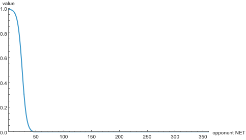
The logistic function \(\mathcal L_{\nicefrac 14}(O, 25)\), used to weight upset wins. Since NET rankings are absolute — i.e. nobody can share a score — this weight doesn’t consider a win an “upset” unless you beat a top-30(ish) team.
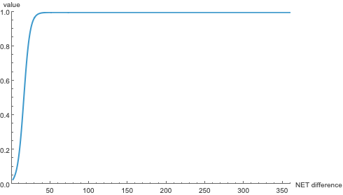
The logistic function \(\mathcal L_{-\nicefrac 14}(O, I+15)\), used to weight upset losses. Basically, the worse your opponent was relative to you, the higher the penalty.
For example, here’s Washington’s after their upset win against Michigan on January 1st. Michgan was ranked 6th in the NET, it was a Big Ten conference game, and it was played at the Hec Ed, Washington’s home court.
| Win/Loss | Conference | Location | Strength | Date |
|---|---|---|---|---|
| \(1\) | \(1\) | \(0.875\) | \(0.991\) | \(0.245\) |
The is then \[ 1 \cdot 1 \cdot 0.875 \cdot 0.991 \cdot 0.245 \approx 0.212, \] so this game contributes \(0.212\) points to Washington’s will-upset . (Another way to look at this is that each game is worth \(1\) point, and Washington got \(\approx 21\%\) of that point in this game. That’s pretty good for a three-month-old game.) Since all the s are bounded between \(0\) and \(1\), teams with more (without loss of generality) will-upset games will probably have more will-upset points. So, if a team has lots of be-upset games, we can look at how many points they earned to judge how likely an upset might be.
From here I make a “fact sheet” for each team summarizing (what I believe are) the statistically important parts of their season, and contributions to their s. Here, for example, is Washington’s:
All told, the s are really just a heuristic to help me decide whether a particular matchup needs more scrutiny. Most of the time, this works. In the women’s tournament, for example, comparing be-upset and will-upset scores helped me catch all three first-round upsets; in the first two rounds, it helped me find three of the four OT games as well. (It may be worth noting that there’s significant overlap between those sets of games.) Through the first round on the men’s side, I identified all upsets except Wisconsin/High Point (there seemed to be very little signal on that one). I also picked other upsets that didn’t come to pass, but we’ll talk about that in the next installment.
(As I’m writing, I’ve just found out that Addie Deal, a five-star freshman at Iowa, is entering the transfer portal. I give up.)