
The study of linear denoising is continued in this section, this time, with the familiar hibiscus image. The image is shown below:
The equation for the photo with noise added to it is: .
Where w is the noise being added to the original photo. The hibiscus with noise added is given below:

The method used to denoise the hibiscus is the same as the one used in the previous section. A Gaussian filter, h, is constructed that is parameterized by it's bandwith, .
After the filter is constructed, we convolve the image with the filter in an attempt to clean the noise from the image. Below is the first filter Mr. Peyrę constructs:

As previously mentioned, Mr. Peyrę proceeds to convolve the noisy hibiscus image with the filter above, and the resulting denoising occurs:

Oof. The filter is too strong. We have lost too much of the original. In the exact same manner as the previous section, Mr. Peyrę uses different values for
. The results are shown below:

Again, Mr. Peyrę iterates through many values for in order to
determine what bandwith parameter would give the best image denoising.

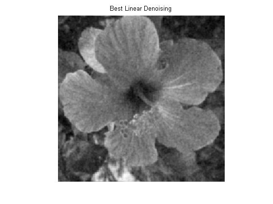
The best value for was determined to be
.8933. Here is the resulting image denoising using .8933 for
.
Wiener Filter is now implemented by Mr. Peyrę. The process is the exact same that it was last time with the signal, except that this time, it is done in two-dimensions. To reiterate,
we again we consider . In the words of
Mr. Peyrę, "We suppose here that
is
realization of of a random vector
, whose
distribution is a Gaussian with a stationary covariance c, and we denote
the power spectrum of
. (1)
Mr. Peyrę proceeds to give the "oracle optimal filter" that minimizes the "risk." The equation for this filter is:
It turns out that the solution to this "oracle optimal filter" is the Wiener Filter. It is given by the equation below:
Where is the variance of the noise.
Mr. Peyrę proceeds to attempt an approximation to the Wiener Filter. is approximated by:
Here is our approximation to the Wiener Filter:
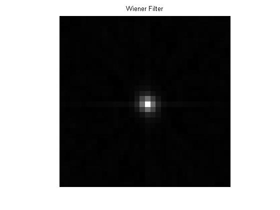
Mr. Peyrę notes that this is a theoretical filter - "in practice one does not have access to ." (2)
Next, we perform a convolution with our filter approximation and the noisy image.

Clearly, both the Linear Denoising and Wiener Filtering were helpful in cleaning up the hibisucus image. Deciding on which of the two did the best job is not so easy. From an aesthetic point of view, I cannot say which of the two is better. If one were to randomly show me the two pictures, I would not be able to discern which one is which. From the results in this section I am beginning to think that denosing is a pretty difficult process, and completely removing all of the noise is not possible. The denoising is very helpful in being able to clean up the noise to a certain degree, but cannot realistically hope to clean all of it. Now, the next section on this topic gets a bit complicated, and covers some topics that I am yet to learn about. Nevertheless, I am still going to attempt to get through the section.
Works Cited
(1) Peryę, Gabriel. "Linear Image Denoising." Linear Image Denoising. N.p., 2010. Web. 15 Aug. 2014.
(2) Peryę, Gabriel. "Linear Image Denoising." Linear Image Denoising. N.p., 2010. Web. 15 Aug. 2014.
G. Peyré, The Numerical Tours of Signal Processing - Advanced Computational Signal and Image Processing, IEEE Computing in Science and Engineering, vol. 13(4), pp. 94-97, 2011.