For this project our group chose to do Reality Check 1, Kinematics of the Stewart platform, loacted on pages 67-69 of our text.
Introduction:
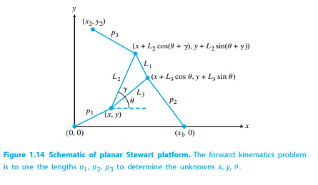
A Stewart platform is normally a three-dimensional platform that has 6 struts that vary in length and move around a platform. However for the sake of this project we dealt with a two dimensional version of the Stewart platform. In this project we wanted to find the postion of the platform given the length of the three struts. Below is an example of the two dimensional version of a Stewart platform that we dealt with.
Here is the work for each of the parts as numbered in the book.
1. For this first part, we used the definitions given in the text to code \(f(\theta)\).
Definition of \(f(\theta)\)
We confirmed that \(f(-\frac{\pi}{4})=0\) and \(f(\frac{\pi}{4})=0\).
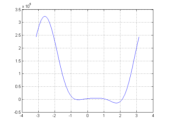
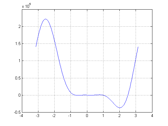
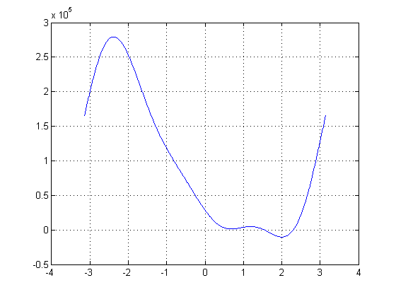
2. We used a slightly modified version of the code for the function \(f(\theta)\) which allowed the function to accept matrix inputs properly so that it could be plotted along with the plot method to achieve this plot of \(f\) on the interval \([-\pi,\pi]\).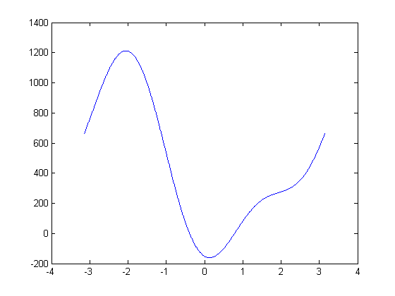
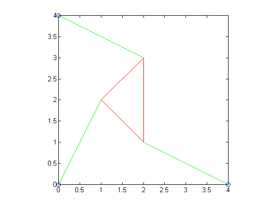
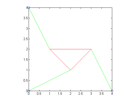
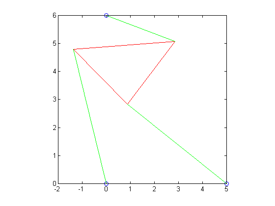
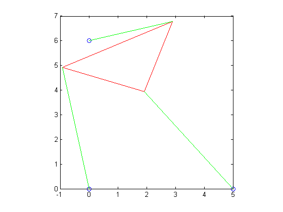
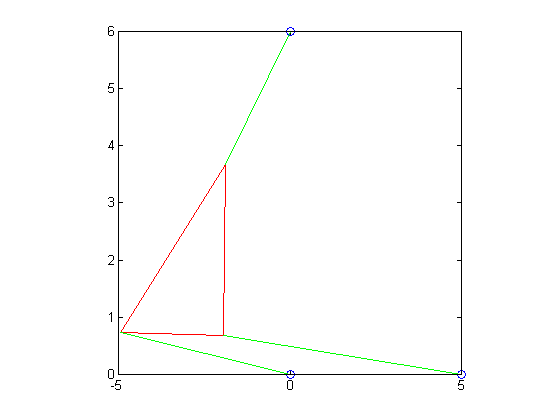
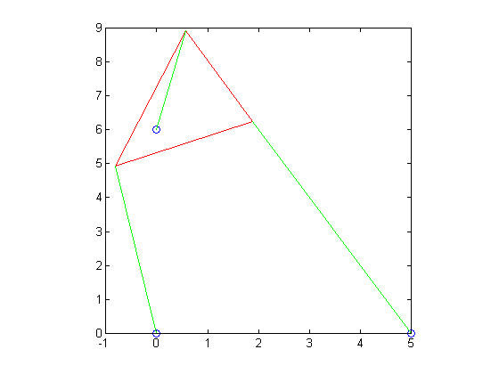
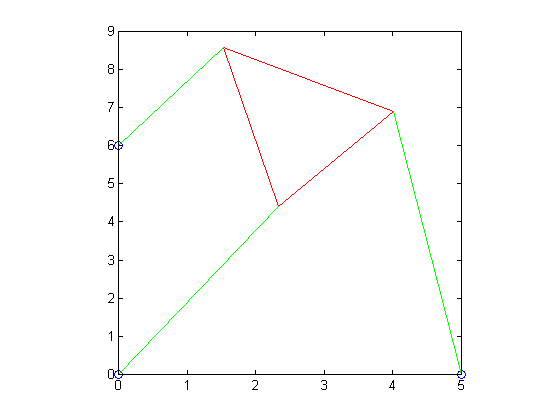
3. We used the plot command as instructed in the text to draw these pictures of the Stewart platform. In addition, we used axis square to force the plot to have a square aspect ratio, so that the plots have an accurate shape.
4. We used the definitions of the kinematics of the platform to create the functions \(g(\theta)\) and \(h(\theta)\), where \((x,y)=(g(\theta),h(\theta))\). Also, we modified the code for drawing the plots of the Stewart Platform to only require the parameters and \(\theta\), so that MATLAB could do the calculations automatically.
We then plotted \(f(\theta)\) and used the plot for approximations of the roots so that we could use fzero to find the roots of \(f(\theta)\).
Finally, we plotted the four poses of the Stewart platform:

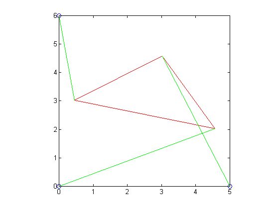
5. We again used the definitions of the kinematics of the platform to create the functions \(g(\theta)\) and \(h(\theta)\), where \((x,y)=(g(\theta),h(\theta))\). Also, we modified the code for drawing the plots of the Stewart Platform to only require the parameters and \(\theta\), so that MATLAB could do the calculations automatically.
We then plotted \(f(\theta)\) and used the plot for approximations of the roots so that we could use fzero to find the roots of \(f(\theta)\).
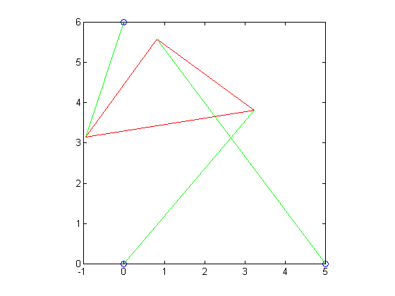
Finally, we plotted the six poses of the Stewart platform:
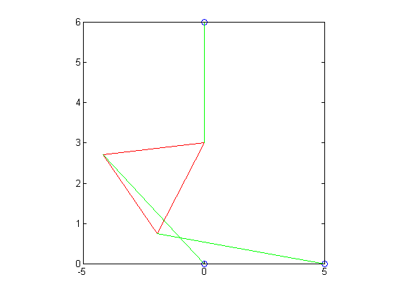

 The two poses being the following:


7. To find the intervals in \(p_2\) that led to \(0,2,4, \text{ or } 6\) poses, we started with an interval in \(p_2\) such that the left side of the interval had, for example, \(0\) roots, and the right side had \(2\) roots. Then we halved the interval so that at each step, the left endpoint had \(0\) roots and the right enpoint had \(2\) roots.
Using this method, we found that the intervals were:
\begin{array}{|c|l|} \hline 0 \text{ poses} & (0,3.70703125 \pm 0.00390625) \\ \hline 2 \text{ poses} & (3.70703125 \pm 0.00390625,4.86328125 \pm 0.00390625) \\ \hline 4 \text{ poses} & (4.86328125 \pm 0.00390625,6.96728515625 \pm 0.00048828125) \\ \hline 6 \text{ poses} & (6.96728515625 \pm 0.00048828125,7.01953125 \pm 0.00390625) \\ \hline 4 \text{ poses} & (7.01953125 \pm 0.00390625,7.84765625 \pm 0.00390625) \\ \hline 2 \text{ poses} & (7.84765625 \pm 0.00390625,9.26171875 \pm 0.00048828125) \\ \hline 0 \text{ poses} & (9.26171875 \pm 0.00048828125,\infty) \\ \hline \end{array}