MATH 447 - Project 4

Objective: Check code by reproducing the results of Example 8.12. First, reproduce the results of Examples 8.13 and carry out Exercise 8.4.4 and Computer Problems 8.4.3. Second, reproduce the results of Example 8.14 and carry out Computer Problem 8.4.4.

Before we go forward it is important to remember that the Dirichlet Boundary Condition (U) specifies the values of the solution itself, while the Neumann Boundary Conditions (Ux) specifies the values that the derivative of a solution is to take on the boundary of the domain.

Burger's Equation General Form:
This equation is a nonlinear equation because of uu_x
It's a simplified model of fluid flow
We'll approximate t(x_i,t_j) by w_ij
We use Dirichlet Boundary Condition \[f(x,t)= \begin{cases} u_t +uu_x=Du_{xx} & \\ u(x,0)= f(x) & \text{for } 0 \leq x \leq 1\\ u(x_{l},t)=l(t) & \text{for all } t \geq 0\\ u(x_{r},t)=r(t) & \text{for all } t \geq 0 \end{cases} \]

Fisher's Equation General Form:
\[f(x,t)= \begin{cases} u_t = Du_{xx} + u(1-u) & \\ u(x,0)= f(x) & \\ u_t(x_{l},t)=l(t) & \\ u_x(x_{r},t)=r(t) & \end{cases} \]

* To understand these formulas a little better, click here.

1. From Burger's to Fisher's Equation
   

   Check code by reproducing the results of Example 8.12.
   Object: To use the Backward Difference Equation with Newton iteration to solve Burgers’ equation
   \[f(x,t)= \begin{cases} u_t +uu_x=Du_{xx} & \\ u(x,0)=\frac{2D\beta\pi\sin(\pi x)}{\alpha + \beta\cos(\pi x)} & \text{for } 0 \leq x \leq 1\\ u(0,t)=0 & \text{for all } t \geq 0\\ u(1,t)=0 & \text{for all } t \geq 0 \end{cases} \]

   
   First, reproduce the results of Examples 8.13 \[f(x,t)= \begin{cases} u_t = Du_{xx} + u(1-u) & \\ u(x,0)=sin(\pi x) & \text{for } 0 \leq x \leq 1\\ u_t(x_{l},t)=0 & \text{for all } t \geq 0\\ u_x(x_{r},t)=0 & \text{for all } t \geq 0 \end{cases} \]

   \(f(x) = 0.5 + 0.5*cos(\pi x)\)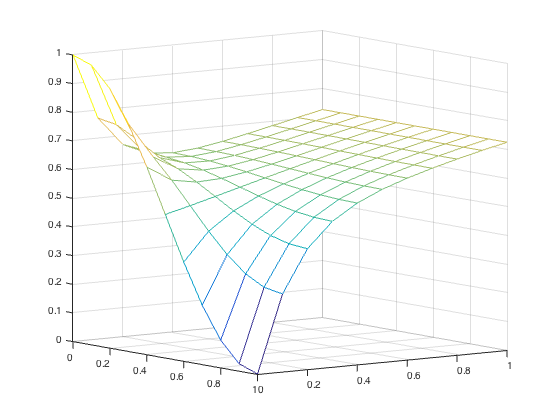

   \(f(x) = 1.5 + 0.5*cos(\pi x)\)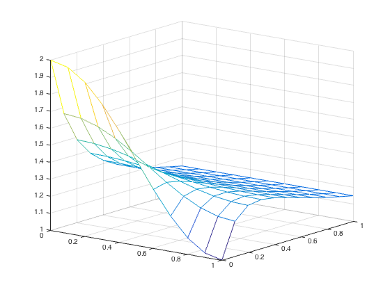

   Carry out Exercise 8.4.4
   Objective:
   Show that fo any constant c, the function u(x,t) = c is an equilibrium solution of Burgers' equation u_t + uu_x = Du_xx.
   f(u) = u(u-1)(2-u);
   f(u) = 3u^2 - u^3 - 2u; f'(u) = 6u - 3u^2 - 2;
   u = 0; (stable)
   u = 1;
   u =2; (stable)
   
   f'(0) = -2;
   f'(1) = 1;
   f'(2) = -2;
   
   Now Compute Problems 8.4.3.
   Plot the approximate solution for \(0 \leq t \leq 2\) for step sizes h = k = 0.05. Which equilibrium solution does the solution approach as time increases?

   \(f(x) = 1/2 + cos(\pi x)\) 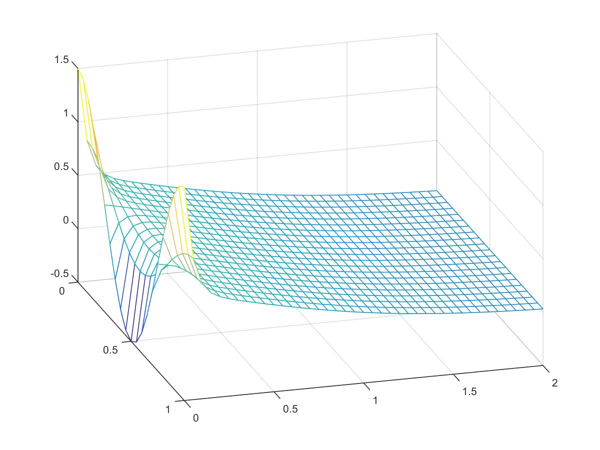Equilibrium solution approaches 0

   \(f(x) = 3/2 - cos(2 \pi x)\) 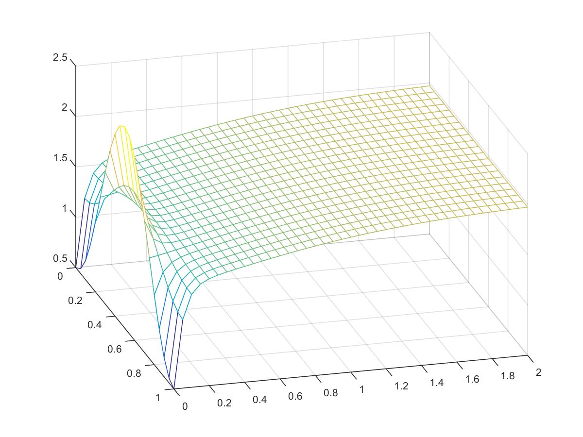Equilibrioum solution approaches 2

   
   
   \begin{align} \frac{w_{ij} - w_{i,j-1}}{k} = \frac{D}{h^2} (w_{i+1,j}-2w_{ij}+w_{i-1,j}) + 3w_{ij}^2-w_{ij}^3-2w_{ij} \\ \end{align} $$Setting: \frac{Dk}{h^2}=\sigma; w_{ij} = z_i; w_{i+1,j}=z_{i+1};w_{i-1,j}=z_{i-1}$$ \begin{align} (2\sigma z_i - 3kz_i +kz_i ^3 + 2kz_i + z_i) - w_{i,j-1}- \sigma z_{i+1} - \sigma z_{i-1} = 0 \\ \frac{dz_i}{dF}= 2\sigma - 3k + 3kz_i ^2k + 1 \\ \frac{dz_{i+1}}{dF} = \frac{dz_{i-1}}{dF} = - \sigma \end{align}

2. Two-Dimentional Fisher's Equation & Graphics
   Reproduce the results of Example 8.14
   Objective: Apply the Backward Difference Method with Newton's iteration to Fisher's equation on the unit squre [0,1] x [0,1]:
   \[f(x,t)= \begin{cases} u_t = D \Delta u + u(1-u) & \\ u(x,y,0)= 2 + cos(\pi x)cos(\pi y) & \text{for } 0 \leq x,y \leq 1\\ u_t(x_{l},t)=0 & \text{for all } t \geq 0\\ u_{n}(x_{r},t)=0 & \text{for all } t \geq 0 \end{cases} \]
   
   Partial Derivative With Respect of Time (Going Backwards):[See Note Here]
   \begin{align} \frac{w_{ij}-w'_{ij}}{dt} = \frac{D}{h^2}(w_{i+1,j}-2w_{ij}+w_{i-1,j}) +\frac{D}{h^2}(w_{i,j+1}-2w_{ij}+w_{i,j-1}) + 3w_{ij}^2 - w_{ij}^3 - 2w_{ij} \\ \frac{w_{ij}}{dF} + \frac{2D}{h^2}w_{ij} + \frac{2D}{k^2}w_{ij} - 3w_{ij}^2 + w_{ij} + 2w_{ij}) - \frac{D}{h^2}(w_{i+1,j}+w_{i-1,j})-\frac{D}{h^2}(w_{i,j+1} + w_{i,j-1})-\frac{w_{ij}}{dt} = 0 \\ \frac{dw_{ij}}{dt} = \frac{1}{dt} + \frac{2D}{h^2} + \frac{2D}{k^2} - 6w_{ij} + 3w_{ij} + 2 \\ \frac{dw_{i+1,j}}{dF} = \frac{dw_{i-1,j}}{dF} = -\frac{D}{h^2} \frac{dw_{i,j+1}}{dF} = \frac{dw_{i,j-1}}{dF} = -\frac{D}{k^2} \end{align}