<- Back to home
Project 5
Project 5
Image Compression using Discrete Cosine Transforms
Patrick Bishop
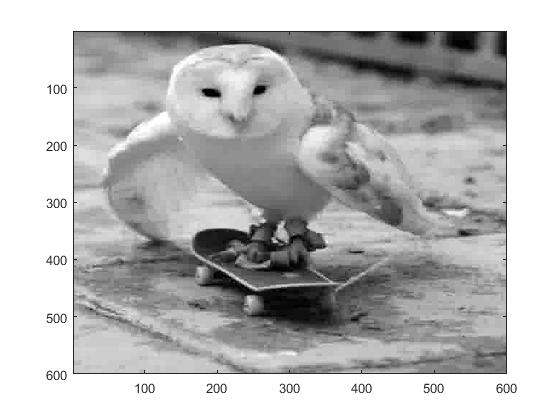
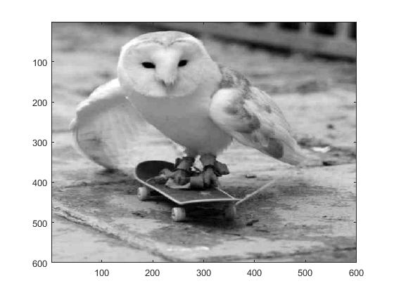
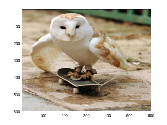
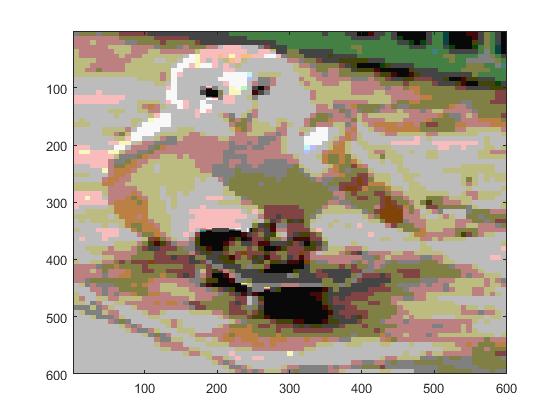
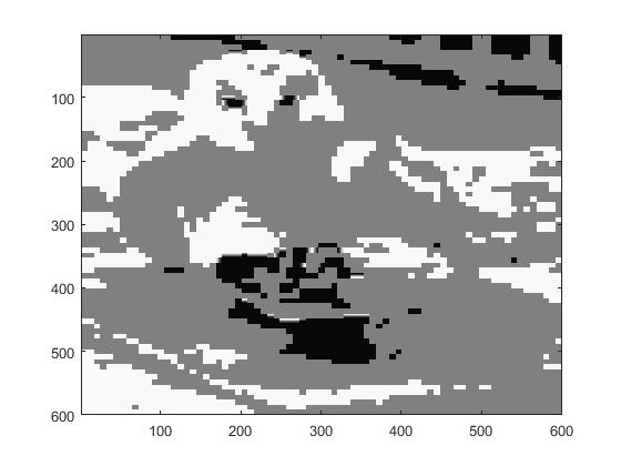
This project focused on image compression techniques using discrete cosine transforms. The guidelines for the project can
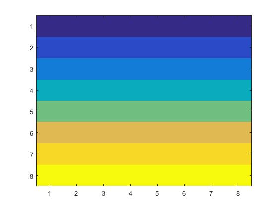
be found here: Project Guidelines . The picture I used to test my programs was the photo below:
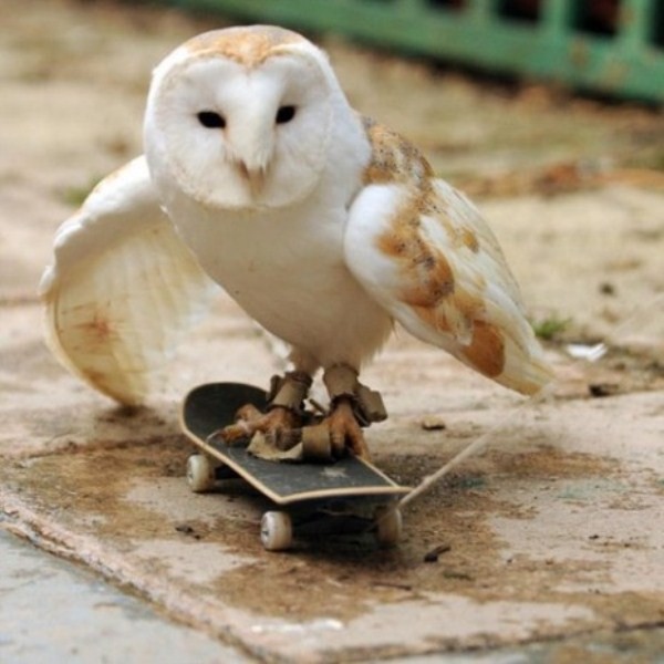

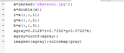
Image Compression using Grayscale Images
For this portion of the project, I took the original color image and converted it into grayscale using the runner code:
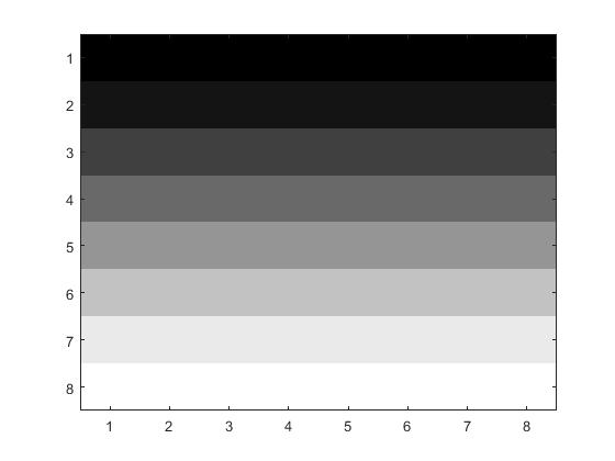
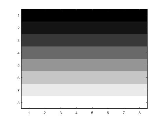
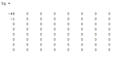
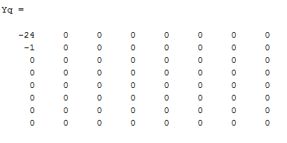
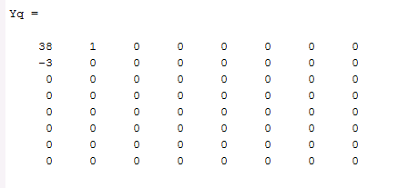
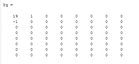
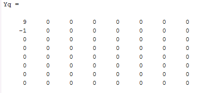
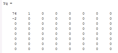
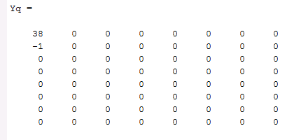
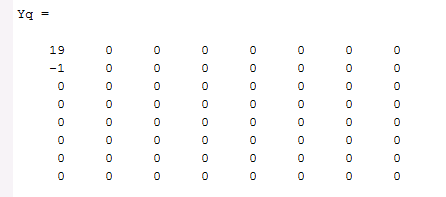
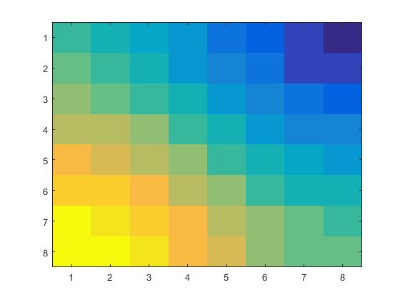
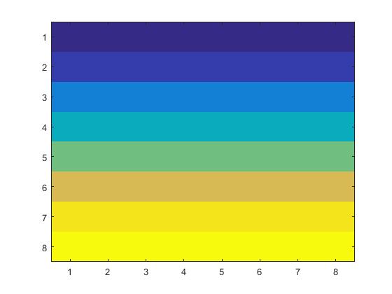
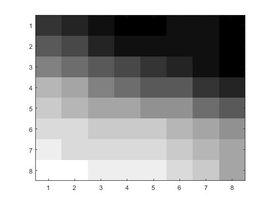
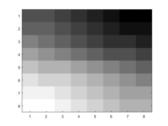
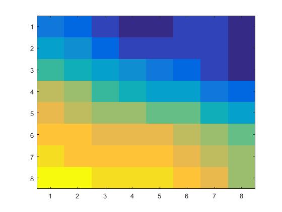
 The first step of the project was to compress an 8x8 grid of pixels and compare how different values of error affect the quality
of the photo when the photo is decompressed. To do this we used the code: DCT.m. The DCT.m program creates a discrete
cosine transform matrix, compresses the 8x8 pixel block, and then uncompresses it. After the picture is uncompressed we can
see that the difference between the two 8x8 pixel blocks is considerably noticable.
The first step of the project was to compress an 8x8 grid of pixels and compare how different values of error affect the quality
of the photo when the photo is decompressed. To do this we used the code: DCT.m. The DCT.m program creates a discrete
cosine transform matrix, compresses the 8x8 pixel block, and then uncompresses it. After the picture is uncompressed we can
see that the difference between the two 8x8 pixel blocks is considerably noticable.
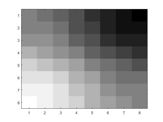
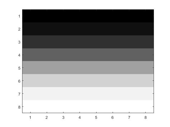
| Before |
After |
 |
 |
The next step was to write code that could compress an entire image. The code I wrote is called dctloop.m and it
it separates the photo into 8x8 bloxks of pixels and sends each block to the dct.m function. I tested out different values of loss parameters, p,
to see how badly the compression would render the grayscale photo. When p=1, there seems to be no sign of distortion in the
picture but at p=4, you can start to see the picture become slightly pixelated.
Quantization with a JPEG Matrix
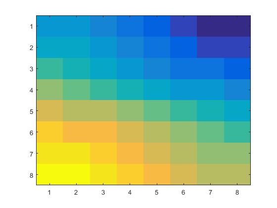
Next, I used the JPEG quantization matrix instead of the linear quantization matrix. Using this matrix in the quantization step,
I tested the program using the grayscale photo and the code dct2.m which is the same code as dct.m but with a
the new quantization matrix. Using this on the 8x8 pixel photo we can see the difference:
| Before Compression |
After Compression |
| |
 |
As in part 1, I ran dctloop.m to compress the entire photo. As the value of p was increased, the clarity of the picture began to degrad but
it still is better than the compression in part 1.
Image Compression of a Color Image (RGB)
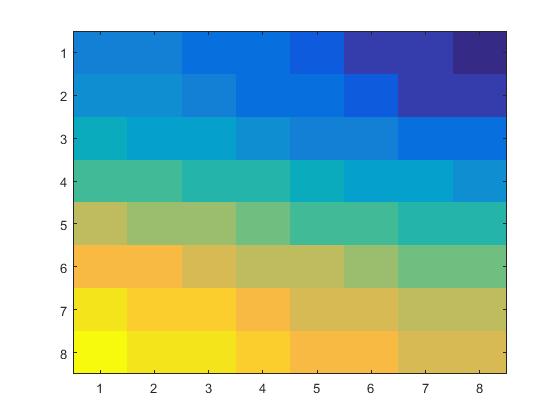
The next step was to compress the color version of this image using the RGB color system. In order to do this, I used the program
sweetandsauer.m to seperate the colors and individually compresses and decompress
them using the function dctcolor.m using the same method as the previous sections. For
the 8x8 pixel block, you can see a some differences after decompression but for the overall picture, the difference seems negligable.
| Before |
After |
 |
 |
Testing out different loss parameters, we see the picture does not suffer very much distortion even with p=4.
Image Compression of a Color Image (YUV Color System/ Baseline JPEG Quantization)
This last problem dealt with using the YUV color system where $Y=0.299R+0.587G+0.114B$, $U=B-Y$, and
$V=R-Y$. For this process, I used the function sweetandsauer2.m to split up and
define the colors. Then I used the function dct2color.m for the luminance, Y, and the function
dct3color.m for the color differences U and V colors to compress and decompress the pictures in the same
manor as before. For the quantization, I send the Y matrix to dctY.m and U and V
to dctUV.m. For the 8x8 block,
| Before |
After |
| |
 |
Testing out different loss parameters, we see the picture does not suffer very much distortion even with p=4.
Final Comparison
For the grayscale image, the JPEG method of quantization produces better quality than the linear method.
But the difference between the two quantization methods is apparent for large values of the loss
parameter. For p=10,
| Linear |
JPEG |
 |
 |
The same goes for the color image. For p=60 we see clearly that the linear method of quantization
is better with large values of p.
| R/G/B |
Y/U/V |
 |
 |