Project 4
Burger's Equation
Group Members: Patrick Bishop, Robert Argus, and Vincent Caetto
The project guidelines can be found here .
The general form for the code we used was: Burger's Equation
Nonlinear Partial Differential Equations are PDEs whose boundary conditions contain functions whose derivatives depend
on more than one independent variable. These types of equations are found in many different fields of science, such as
fluid mechanics, thermodynamics and relativity, among others. As NPDEs contain partial derivatives that rely on more than
one variable, we cannot simply solve them using the "centered-difference" formulas. Instead, we have to apply finite
difference approximations to the individual partial derivates. By using the Newton's Method, we can calculate the
"backward-difference" equations and evaluate them at each step to find the corresponding values for our variables at said
step. An example of a nonlinear partial differential equation is Burger's equation.
Reconstruction of Example 8.12: Solving Burger's Equation
Burger's Equation is an elliptic equation describing a simplified model for fluid flow. It is given by:
$$u_t + uu_x = Du_{xx} \quad \quad (1) $$
It is evident that Burger's Equation is nonlinear, as the \(uu_x\) term relies on a product of the function and a
partial derivative. We can use Burger's Equation to form a set of boundary equations for our nonlinear PDE:
\[\begin{cases} u_t + uu_x = Du_{xx} \\ u(x,0) = f(x) \\ u_x(x_l,t) = l(t) \\ u_x(x_r,t) = r(t) \end{cases}\]
This set of conditions is known as Dirichlet boundary conditions. Using these conditions, we can then use Multivariable
Newton's method to get:
\[ \frac{w_{ij}-w_{i,j-1}}{k} + w_{ij}\frac{w_{i+1,j}-w_{i-1,j}}{2h} - D\frac{w_{i+1,j}-2w_{ij}+w_{i-1,j}}{h^2} = 0\]
This "backward-difference" equation lets us solve for \(w_{ij}\),\(w_{i+1,j}\) and \(w_{i-1,j}\) at each time step j.
The j-1 refers to the data from the previous step, letting us extend the time to any limit we choose. We can also rewrite
this equation, by setting \(\vec{Z} = [w_{ij},...,w_{mj}]\), where m is the number of unknowns. Using this conversion,
we get:
\[ \vec{Z}^{k+1} = \vec{Z}^k - DF(\vec{Z}^k)^{-1}F(\vec{Z}^k) \]
By iterating this equation, we can find our final values for each \(w_{ij}\).
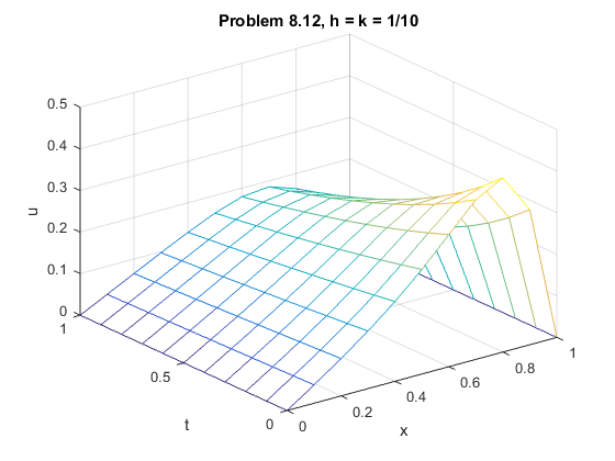
We then used these methods illustrated above to reconstruct Example 8.12 and solve Burger's equation with Dirichlet
Boundary conditions. Given the set of equations:
\begin{eqnarray*}
u_t + uu_x = Du_{xx} \\
u(x,0) = \frac{2D\beta \pi \sin{\pi x}}{\alpha + \beta \cos{\pi x}}, 0 \leq x \leq 1 \\
u(0,t) = 0, \forall t \geq 0 \\
u(1,t) = 0, \forall t \geq 0
\end{eqnarray*}
We set $\alpha = 5$, $\beta = 4$, and $ D= 0.05$, as seen in the code here. This produced the result below:
Exercise 8.4.3: Solutions to Burger's Equation
Given that $u(x,t) = -\dfrac{2 \pi \beta e^(D^2 \pi ^2 t) \sin(\pi x)}{\alpha -\pi ^2 \beta e^(D t) \cos(\pi x)}$,
we plugged this equation into (1) and got,
\begin{eqnarray*}
-\frac{2 \pi ^3 \alpha \beta D^2 e^{\pi ^2 D t} \sin (\pi x)}{\left(\alpha e^{\pi ^2 D t}+\beta \cos (\pi x)\right)^2} + \frac{4 \pi ^3 \beta ^2 D^2 \sin (\pi x) \left(\alpha e^{\pi ^2 D t} \cos (\pi
x)+\beta \right)}{\left(\alpha e^{\pi ^2 D t}+\beta \cos (\pi x)\right)^3} &= \frac{2 \pi ^3 \beta D^2 \sin (\pi x) \left(\alpha ^2 \left(-e^{2 \pi ^2 D t}\right)+\alpha \beta e^{\pi ^2 D t} \cos (\pi x)+2 \beta ^2\right)}{\left(\alpha e^{\pi ^2 D t}+\beta \cos (\pi x)\right)^3}\\
\frac{2 \pi ^3 \beta D^2 \sin (\pi x) \left(\alpha ^2 \left(-e^{2 \pi ^2 D t}\right)+\alpha \beta e^{\pi ^2 D t} \cos (\pi x)+2 \beta ^2\right)}{\left(\alpha e^{\pi ^2 D t}+\beta \cos (\pi x)\right)^3} &= \frac{2 \pi ^3 \beta D^2 \sin (\pi x) \left(\alpha ^2 \left(-e^{2 \pi ^2 D t}\right)+\alpha \beta e^{\pi ^2
D t} \cos (\pi x)+2 \beta ^2\right)}{\left(\alpha e^{\pi ^2 D t}+\beta \cos (\pi x)\right)^3} \\
\end{eqnarray*}
Since the left side and the right side of the equation agree, the given form for $u(x,t)$ is a solution to
Burger's equation.
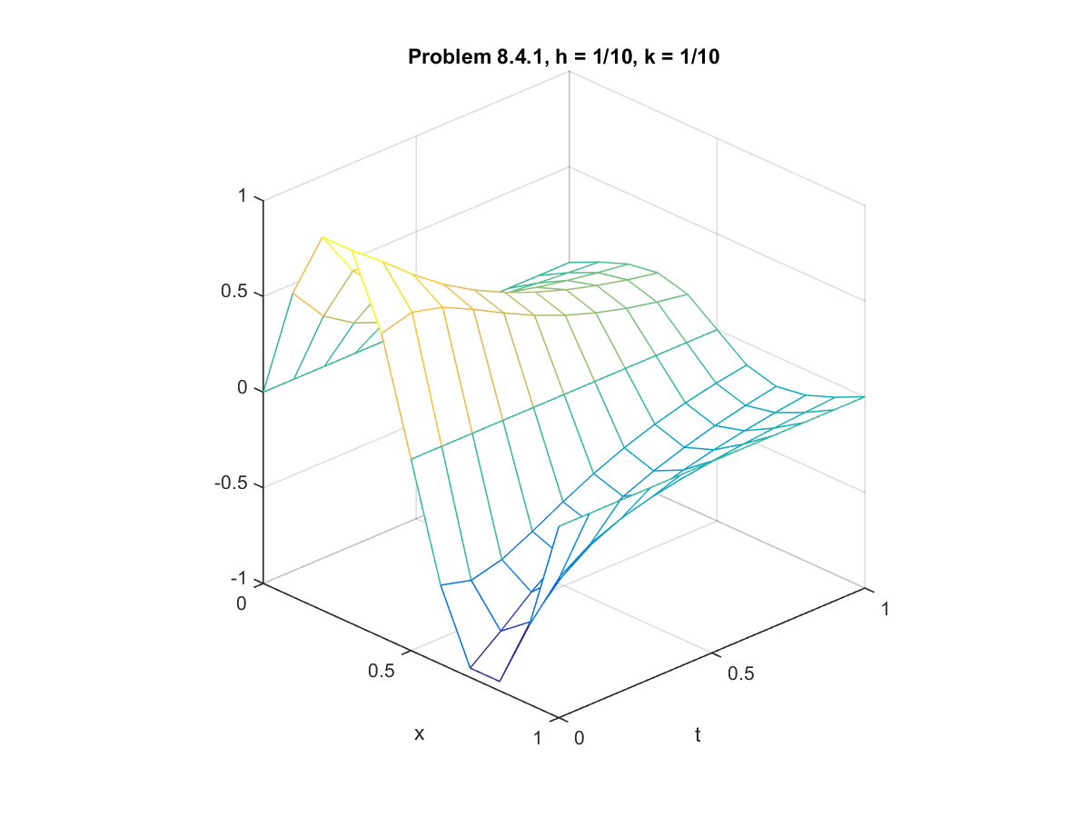
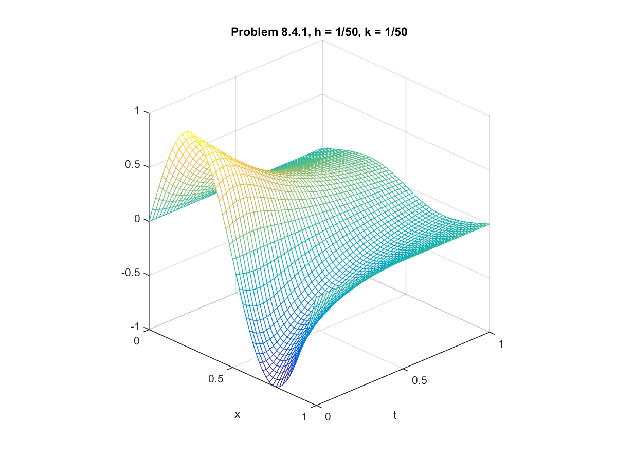
Computer Problem 8.4.1: Equilibrium Solutions to Burger's Equation
For this problem, we solved Burger's equation in a similar manner as before but with different conditions. The conditions were:
\begin{eqnarray*}
f(x) = \sin(2 \pi x) \\
l(t) = r(t) = 0
\end{eqnarray*}
For part a we used step sizes $h=k=0.1$, and for part b we used step sizes $h=k=0.02$. The code adapted to handle this scenerio can be found here. The plots of the solutions can be found below.
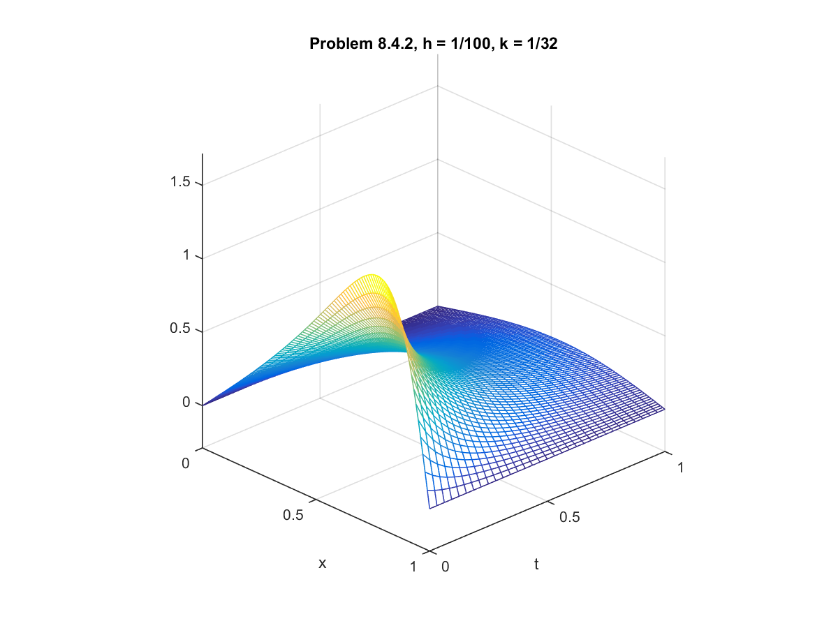
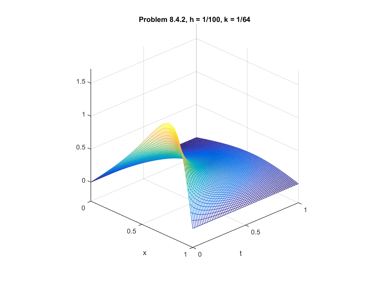
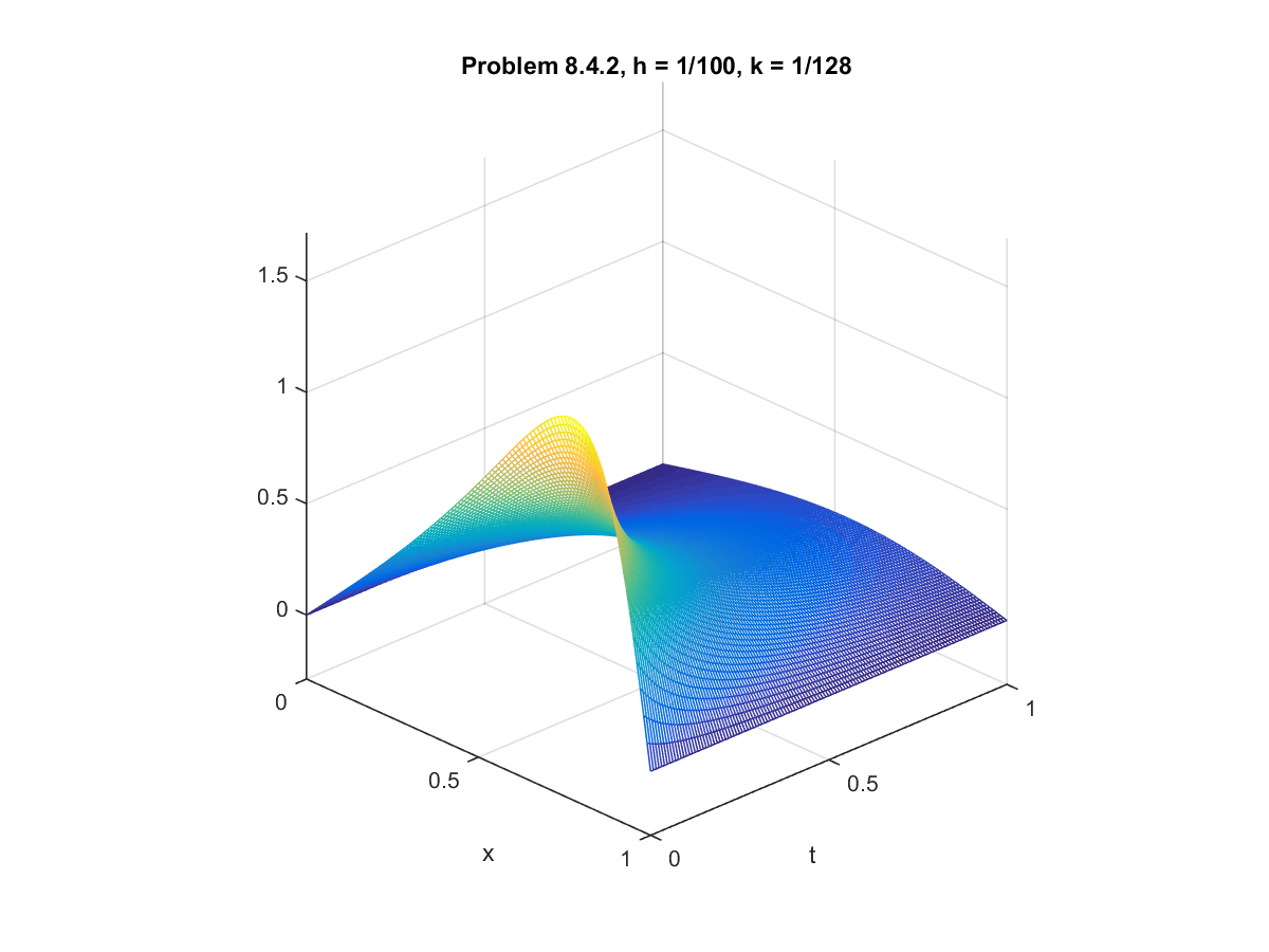
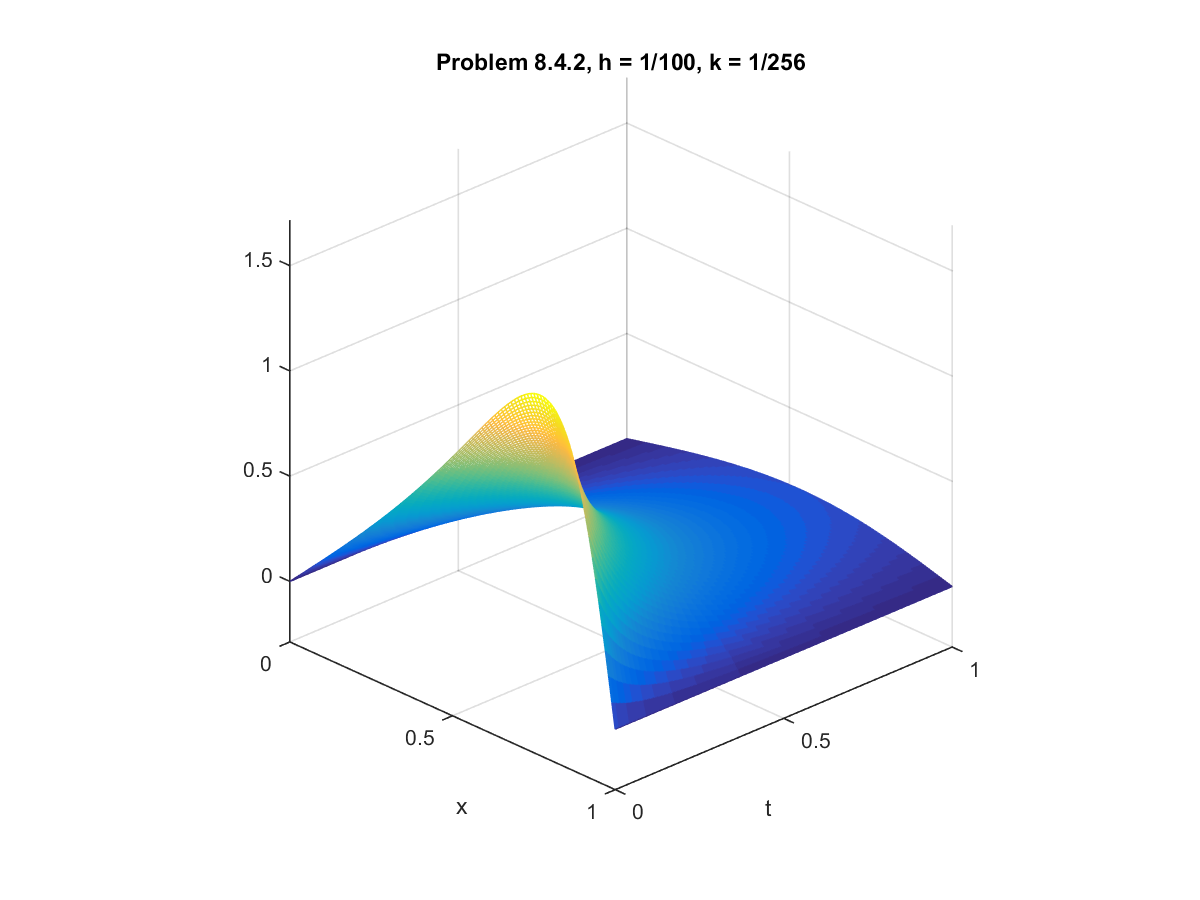
Computer Problem 8.4.2: Burger's Equation with Homogeneous Dirichlet Boundary Conditions
For this problem, we use the conditions from example 8.12 but with different values for the constants. We set
$\alpha = 4$, $\beta = 3$, and $D = 0.2$. We fixed the step size $h = 0.01$ and compared solution sets for
various step sizes for $k$.
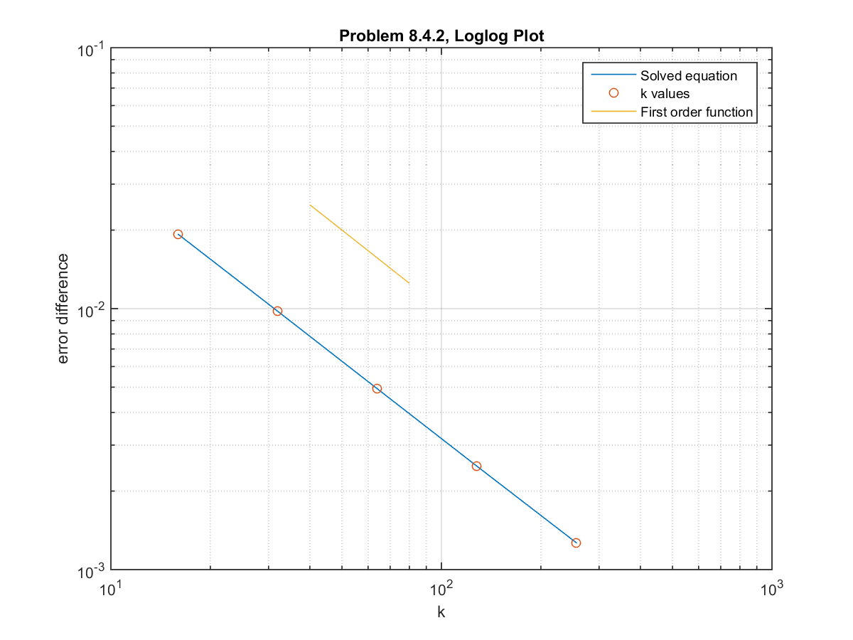
The relationship between the error difference and the $k$ value is near a first order relationship, as seen by the log-log plot below.
The actual slope of the log-log plot is -0.9820
<- Back to home