GPS Analysis: Collins, Sarkhel, Smith

GPS, Conditioning, and Nonlinear Least Squares

Stephen Collins, Kunal Sarkhel, Mezel Smith

Overview

Utilizing matrix conditioning, geometry, and least squares, this project investigates the quantitative machinery running the Global Positioning System (GPS).At all times, GPS allows receivers located at any point on earth access to accurate, synchronized signals from five to twelve atomic clocks in satellites orbiting at predetermined locations. For the receivers to accurately pinpoint their own respective locations, there must be mathematical consideration on the various factors (such as signal interference and distances between satellites) that could affect when and where the receiver gets the signals after the signal has already been sent.

Activity I: Locating a Receiver

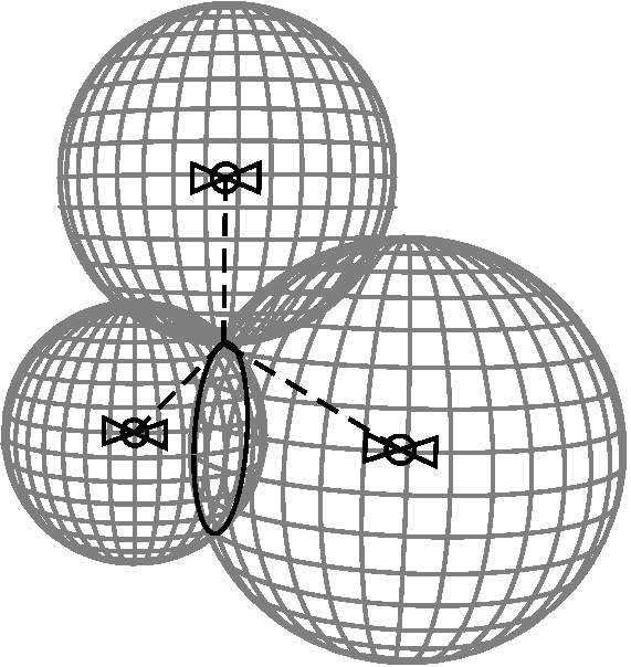
Suppose we had $n$ satellites, where the i$^{\text{th}}$ satellite had a cartesian position of $ \left(A_i,B_i,C_i\right) $. Then, we can imagine a sphere whose radius $R_i$ is the distance between the receiver and the i$^{\text{th}}$ satellite. By considering the speed of the signal $c \approx 299792.458 \frac{\text{km}}{\text{s}}$, the time $t_i$ it takes for the receiver to get the signal, and the difference $d$ between the reciever's clock and the satellite's atomic clock, we have that $R_i = c\left(t_i - d \right) $. With this formulation, we can determine the location of the receiver by finding the intersection all $n$ spheres.

(Courtesy of www.gnns.be/how_tutorial.php)

This equates to solving the system of $n$ nonlinear equations, where any equation is as follows: \[f_i(x,y,z,d) = (x-A_i)^2 + (y-B_i)^2 + (z-C_i)^2 - \left(c(t_i - d)]\right)^2 = 0\] In euclidean space, intersecting spheres may at most intersect at two locations, but in the context of this situation, one possible solution will seem far from Earth. So now we consider having four satellites. Letting $v = (x,y,z,d)$, and $F(v)$ be a matrix of the $f_i$ functions, then using multivariate Newton's Method allows iteration from an initial guess $v_0$ toward the function's $F$ two possible roots; and thus, the two possible locations of the receiver. The computationally efficient form of the method found in section 2.7 of the textbook (pg. 132) is:

\begin{align} DF(v_k)s&=-F(v_k)\\ v_{k+1}&=v_k+s \end{align}

Where, the vector valued function $F(v)$ and the Jacobian matrix $DF(v)$ are explicitly defined as:

\begin{align} F(v) &= \begin{bmatrix} f_1(x,y,z,d)\\ f_2(x,y,z,d)\\ f_3(x,y,z,d)\\ f_4(x,y,z,d) \end{bmatrix}\\\\ DF(v) &=\begin{bmatrix} \frac{\partial f_1}{\partial x} & \frac{\partial f_1}{\partial y} & \frac{\partial f_1}{\partial z} & \frac{\partial f_1}{\partial d}\\ \frac{\partial f_2}{\partial x} & \frac{\partial f_2}{\partial y} & \frac{\partial f_2}{\partial z} & \frac{\partial f_2}{\partial d}\\ \frac{\partial f_3}{\partial x} & \frac{\partial f_3}{\partial y} & \frac{\partial f_3}{\partial z} & \frac{\partial f_3}{\partial d}\\ \frac{\partial f_4}{\partial x} & \frac{\partial f_4}{\partial y} & \frac{\partial f_4}{\partial z} & \frac{\partial f_4}{\partial d} \end{bmatrix} \end{align}

The partial derivatives of $f_i$ are:

\[\begin{array}{cccc} \frac{\partial f_i}{\partial x}= 2(x - A_i), & \frac{\partial f_i}{\partial y} = 2(y - B_i), & \frac{\partial f_i}{\partial z} = 2(z - C_i), & \frac{\partial f_i}{\partial d} = 2c^2(t_i - d) \end{array} \]

From there, Guassian elimination will approximate the root in $\frac 2 3 n^3 \approx 43$ operations per iteration. After implementing multivariate Newton's Method as a MATLAB function (newtgps), we tested it using the sample data.

Satellite Data

$A$	$B$	$C$	$t$
$15600$	$7540$	$20140$	$0.07074$
$18760$	$2750$	$18610$	$0.07220$
$17610$	$14630$	$13480$	$0.07690$
$19170$	$610$	$18390$	$0.07242$

Initial Vector $v_0$

$x_0$	$y_0$	$z_0$	$d_0$
$0$	$0$	$6370$	$0$

Expected Near Earth Solution

$x$	$y$	$z$	$d$
$-41.77271$	$-16.78919$	$6370.0596$	$-3.201566 \times 10^{-3}$

The function successfully approximated both solutions. In the case of the near earth solution, this was to all digits of accuracy given. The distant solution was compared to the result of activity 2 to gauge its accuracy.

Multivariate Newton's Method Results

$x$	$y$	$z$	$d$	Iterations
$-41.772709570873$	$-16.789194106532$	$6370.059559223340$	$-3.201565830 \times 10^{-3}$	$10$
$-39.747837348212$	$-134.274144360682$	$-9413.624553735810$	$ 0.185173047096$	$10$

Activity II: Finding Reciever Location Via Quadratic Equation

To verify the results from activity I, we can determine the two possible solutions by turning the function $f_1=f_1(d)$ of degree two in $d$. Subtracting $f_2,f_3,f_4$ from $f_1$ yields three linear equations in the form \[x \vec{u}_x + y \vec{u}_y + z \vec{u}_z + d \vec{u}_d + \vec{w} = 0\]

Expanding $f_i$ gets us \[x^2-2A_ix+A_i^2+y^2-2B_iy+B_i^2+z^2-2C_iz+C_i^2=c^2 t_i^2 -2c^2t_id + c^2 d^2\] If we subtract any equation $f_j$ from $f_1$, then our result is: $$(2A_j-2A_1)x+(2B_j-2B_1)y+(2C_j-2C_1)z + 2c^2(t_j - t_1) d + \left( c^2(t_j^2 - t_1^2)+\left(A_1^2+B_1^2+C_1^2\right) - \left(A_j^2+B_j^2+C_j^2\right) \right) =0 $$ It becomes clear what the parametric vector form of the system of equations becomes:

Where, if we consider the components of the vectors, we have that: \begin{align} \vec{u}_x(i) &= 2\left(A_i-A_1\right)\\ \vec{u}_y(i) &= 2\left(B_i-B_1\right)\\ \vec{u}_z(i) &= 2\left(C_i-C_1\right)\\ \vec{u}_d(i) &= 2 c^2\left(t_i-t_1\right)\\ \vec{w}(i) &= c^2(t_i^2 - t_1^2)+\left(A_1^2+B_1^2+C_1^2\right) - \left(A_i^2+B_i^2+C_i^2\right) \end{align}

Referring back to the parametric-vector form equation, because this equation is a vector sum equal to zero, any matrix including it as a column will also have a determinant equal to zero. The textbook utilizes this fact to construct just such a determinant allowing $x$ to be expressed in terms of $d$, after some further manipulation using other determinant properties, we arrive at:

\begin{align} 0&=det[\vec u_y|\vec u_z|x\vec u_x+y\vec u_y+z\vec u_z+d\vec u_d+\vec w]\\\\ 0&=det[\vec u_y|\vec u_z|x\vec u_x]+det[\vec u_y|\vec u_z|y\vec u_y] + det[\vec u_y|\vec u_z|z\vec u_z]+det[\vec u_y|\vec u_z|d\vec u_d] + det[\vec u_y|\vec u_z|\vec w]\\\\ 0&=xdet[\vec u_y|\vec u_z|\vec u_x]+ydet[\vec u_y|\vec u_z|\vec u_y] + zdet[\vec u_y|\vec u_z|\vec u_z]+ddet[\vec u_y|\vec u_z|\vec u_d] + det[\vec u_y|\vec u_z|\vec w]\\\\ 0&=xdet[\vec u_y|\vec u_z|\vec u_x]+0+0+ddet[\vec u_y|\vec u_z|\vec u_d] + det[\vec u_y|\vec u_z|\vec w]\\\\ -xdet[\vec u_y|\vec u_z|\vec u_x] &= ddet[\vec u_y|\vec u_z|\vec u_d] + det[\vec u_y|\vec u_z|\vec w]\\\\ \end{align}

\begin{align} x&=\left(-\frac{det[\vec u_y|\vec u_z|\vec u_d]} {det[\vec u_y|\vec u_z|\vec u_x]}\right)d +\left(-\frac{det[\vec u_y|\vec u_z|\vec w]} {det[\vec u_y|\vec u_z|\vec u_x]}\right) = m_xd+b_x \end{align}

Formulas for $y$ and $z$ in terms of $d$ can be obtained in a similar fashion.

\begin{align} y&=\left(-\frac{det[\vec u_x|\vec u_z|\vec u_d]} {det[\vec u_x|\vec u_z|\vec u_y]}\right)d +\left(-\frac{det[\vec u_x|\vec u_z|\vec w]} {det[\vec u_x|\vec u_z|\vec u_y]}\right) = m_yd+b_y\\\\ z&=\left(-\frac{det[\vec u_x|\vec u_y|\vec u_d]} {det[\vec u_x|\vec u_y|\vec u_z]}\right)d +\left(-\frac{det[\vec u_x|\vec u_y|\vec w]} {det[\vec u_x|\vec u_y|\vec u_z]}\right) = m_zd+b_z \end{align}

Substituting back into $f_1$, expanding, then grouping like terms yields the following equation:

\[f_1=(m_x^2+m_y^2+m_z^2-c^2)d^2 + 2[m_x(b_x-A_1)+m_y(b_y-B_1)+m_z(b_z-C_1) + c^2t_1]d + [(A_1-b_x)^2+(B_1-b_y)^2+(C_1-b_z)^2-c^2t_1^2] = 0\]

Which can be solved using the Quadratic Formula. Solutions for the other variables immediately follow from the slope-intercept formulas above. After translating this process into MATLAB code (quadgps) we evaluated the function using the same sample data as in step one with nearly identical results.

Quadratic Formula Results

$x$	$y$	$z$	$d$
$-41.772709570837$	$-16.789194106527$	$6370.059559223344$	$-3.201565830 \times 10^{-3}$
$-39.747837348143$	$-134.274144360666$	$-9413.624553735753$	$0.185173047096$

We note that we had an alternative location-finding code(quasol) that determined and extracted the coefficients of the $d$ polynomial, and plugged them into the quadratic formula. But due to the purpose of mathematically analyzing the activity, we present with everything above.

Activities IV-V: Transmission Time-Shifts' Effects on Location Accuracy

For our conditioning tests, we convert our satellites to spherical coordinates in order to establish a better geometrical grasp of where the satellites are with respect to Earth. We set the true position of our receiver to be at $ \left(0,0,6730\right)$ with $d=0.0001$. From here, we set the true time it took for the receiver to pick up the signal from the $i^{\text{th}}$ satellite to be $t_i=d+\frac{R_i}{c}$, where $R_i$ is the distance between satellite $i$ and this true location of the receiver. To test the accuracy, we investigate the effects of perturbing the times it seems (which may be due to other physical factors) to take for the reciever to pick up the signals by some $\Delta t_i \approx \pm 10^{-8}$ seconds. Once the times have been slightly shifted, we utilize Newton's Multivariate Method to determine the where the receiver believes it's location is now in comparison to the true location. From here, we can determine the ratio of forward position error to backward position error. Going through a variety of permuations of which satellites get negative and positive time shifts, we arrive at a maximum position error and error magnification factor.

Utilizing MATLAB, we coded a program (testgps) that will go through all these possible $\Delta t_i$ perturbations and then determine the max emf and forward error. We did these tests on four unbunched, and bunched(close-angled with respect to spherical coordinates), satellites. The results were:

GPS Conditioning Results

Configurations	Max Fwd Error (m)	Max EMF
Unbunched	$9.32975837895356 $	$3.11207241209302$
Bunched	$69,950.2353431099$	$23332.8869611222$

Based on the above results, we notice a significant difference in accuracy. Using the same style of perturbation in signal retrieval times, four bunched satellites results in extremely inaccurate results by about 70 kilometers, in comparison to four unbunched satellites, only resulting in a loss of accuracy by a few meters ($ \approx 9 $ m).

Activity VI:Number of Satellites' Effects on Location Accuary

We are aware that from any point on Earth, five to 12 satellites are visible for signal transmission; however, there is a greater chance that considering more than four spheres, if there will exist an actual intersection where the receiver should be located. So here in order to determine the approximate location of the receiver, we utilize a nonlinear least squares method known as the Guass-Newton method. We note that computationally, the code used in all earlier activities that used Newton's Multivariate Method. So we produced a MATLAB function (CheckMultSat) that will iterate conditioning tests from 4 to 12 satellites, plot the emf and fe of each test, and print out the least and most accurate (considering perturbations of the trasnmission times) configuration of all the tests. To keep some consistency, for each number of satellites, we evenly spaced them out with respect to the angular ranges of $\phi$ and $\theta$. The following plots show what the forward errors and emf were for each number of satellites:

It is expected that these plots were familiar in shape, as the EMF is directly proportional to the forward error by a proportionality factor of $\frac{1}{c\Delta t_i}$. Furthermore from these results we can see that:

Multiple-Satellite-Check Results

	Number of Satellites Used	Max Fwd Error (m)	Max EMF
Least Accurate Configuration	$6 $	$9.54523873497237$	$ 3.18394892208141$
Most Accurate Configuration	$10 $	$8.84442267033592$	$2.95018184558062$

This means based on our initial position vector, and the distribution of our satellites, if we add 6 satellites to our originally configuration of 4, we can increase our accuracy (subject to transmission time shifts) to a slight bit more than just having 4 satellites. However, adding only two more satellites creates a situation where transmission time perturbations can result in the least accurate determination of the receiver's position. Overall, we notice that keeping the satellites evenly (with respect to spherical angles) spaced shows promising accuacy; for an error of about 10 meters is still not that bad in comparison to an error of 70,000 (which is preciesly what bunched up satellites provided).