Image Manipulation and Compression with Fourier Analysis and Wavelets via Gabriel Peyrè

In this section I will be using the image of a brain, which Mr. Peyre uses. Again, the links to Mr. Peyrè's work can be found here:

Valuable Links Here

Here is the picture of the brain that Mr. Peyrè uses:

I am going to re-hash the equations for Wavelets, courtesy of Mr. Peyrè's website:

"The forward wavelet transform computes the set of inner products: " (1)

"Where the Wavelet atoms are defined as: " (2)

Now we commence with the wavelet transform of the brain image. Below are the Wavelet coefficients of the brain.

Again, a non-linear hard-thresholding is implemented. This time, T is equal to .5. This method was dicussed previously and Part II, and I am not going to explain it again. Below, the orignal and filtered versions of the wavelet coefficients are given.

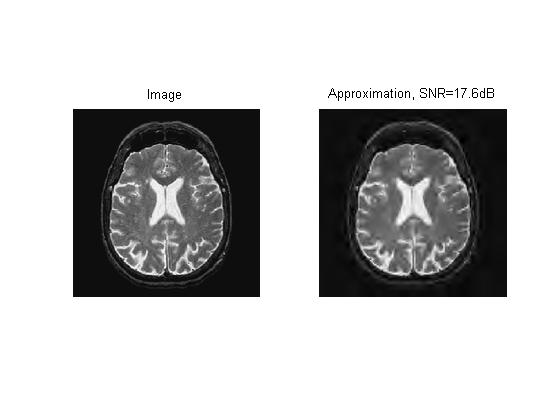
Now, the image is reconstructed with the filtered wavelet coefficients. The results are below:

I can definitely notice a difference between the two images. A considerable degree of clarity is lost, and the SNR is 17.6dB, which is not very good. However, one of the main ideas of Mr. Mallat's book is the idea of sparse representations. The filtered image of the brain is a textbook example of a sparse representation in signal processing. The vast majority of the elements in the matrix of the image are zero. From this perspective, the filtered result is not so terrible. Many of the Wavelet coefficients have been wiped out, and the image is still very discernable. The Huffman Coding for the filtered image would be much more compact than the original one.

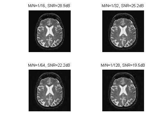
Mr. Peyrè then implements a method whereby a certain number of coefficients are kept. I can imagine this being very useful for applications. Perhaps I'd like a slightly better version of my filtered image, and this could be a means of doing that. Mr. Peyre introduces a method in which 1/16, 1/32, 1/64, and 1/128 of the Wavelet coefficients are retained. As one might expect, as the number of coefficients retained is lowered, the overall quality of the image does is lowered as well.

The first two images are very interesting! Look how the quality is still very good, with just 1/16th of the wavelet coefficients. Even using 1/32nd of them is not bad. Again, this takes us back to the idea of sparse representations in signal processing.

Here, thresholding is again used to clean an image that has had noise to it. Consider noise to be some kind of intereference...junk basically. Can we remove it? Mr. Peyre applies noise "w" to the image "f" yielding y = f = w. (3) The denoiser attempts to reconstruct the image from the messy image. Of course, being mathematicians/engineers, people want a way of quantifying the ability of the denoiser. This is given by the average risk equation:

(4)

Where f~ is the "cleaned-up" image.

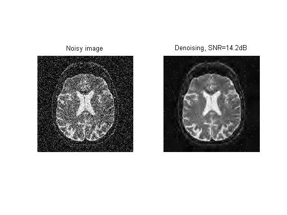
Now, in this setting we have access to the original image. In a real life application, one would probably only have the noisy image, so one would not be able to compute this difference. With this in mind, Mr. Peyre proceeds to add noise to the brain image:

How to clean this mess up? The answer is thresholding, which I have shown several times in my studies of Mr. Peyre's code. According to Mr. Peyre, "The asympototically optimal threshold of Donoho and Johnstone is . (5) He follows this by saying that (6), or roughly three sigma is better in practice. (6) With this number for sigma, hard thresholding is implemented, and the image is reconstructed. First the coefficients are given:

Not bad! This is a simple example, I can imagine in real life it would be more difficult for the reason that we would not know his value for signma either. It would take a bit more trial and error. For fun, I increased sigma to .2. As one might expect, the reconstruction suffers in quality, but does clean up a lot of the noise from the image.

It is also worth noting that T = 3 sigma is an appoximation. One can determine the optimal value by testing many values on an closed interval for T, such as T = [2.5,4], performing the reconstruction, and calculating the subsequent SNR. As always, Mr. Peyre provides code for this. The plot of this relationship between T/sigma and SNR is given below.

With some handy Matlab functions, I was able to determine that the best value for T occurs at 3.3379310. Would this give an improvement over 3?

Indeed, this offers a slight improvement.

Here, an understanding of translation invariance and periodic shifting is required. It is pretty spectacular. This method takes the image you want to denoise, and performs periodic shifting of it. After each shift, the image is then denoised, then shifted back. After this, the image is rebuilt by accumulating the shifted and cleaned up version. It is given by the following formula:

Note: I had issues formatting this correctly and there are mistakes I could not resolve in the codecogs website. Please seek Mr. Peyre's website for the correct version.

Formula formatting issues aside, one can still get the general idea from here. This process is done iteratively - after each shift and denoising, the cleaned up shifted image is placed back into an image which is initialized at zero. Notice how as the shifts get bigger, the image changes are smaller due to the larger denominator it gets at each iteration. This method is fascinating and very cool. The resulting image from this intriguing process is given below:

Wow! Look at this. At the noise is gone. Spectacular!

The end of this section was quite amazing, in my opinion. In fact, I would say the same about most of the rest of this section as well. Mr. Peyrè does an excellent job of building one's intuition with Wavelets with his simple examples. As I have mentioned previously, having access to Mr. Peyrè's code is a huge help to me. Being able to study it is an incredible resource. Next, the 1-D Haar Transform is studied.

• Home
• Part IV: 1-D Haar Wavelets

Works Cited

(1) Peyrè, Gabriel. "Image Processing with Wavelets." Image Processing with Wavelets. N.p., n.d. Web. 29 May 2014.

(2) Peyrè, Gabriel. "Image Processing with Wavelets." Image Processing with Wavelets. N.p., n.d. Web. 29 May 2014.

(3) Peyrè, Gabriel. "Image Processing with Wavelets." Image Processing with Wavelets. N.p., n.d. Web. 29 May 2014.

(4) Peyrè, Gabriel. "Image Processing with Wavelets." Image Processing with Wavelets. N.p., n.d. Web. 29 May 2014.

(5) Peyrè, Gabriel. "Image Processing with Wavelets." Image Processing with Wavelets. N.p., n.d. Web. 1 June 2014.

(6) Peyrè, Gabriel. "Image Processing with Wavelets." Image Processing with Wavelets. N.p., n.d. Web. 1 June 2014.

G. Peyré, The Numerical Tours of Signal Processing - Advanced Computational Signal and Image Processing, IEEE Computing in Science and Engineering, vol. 13(4), pp. 94-97, 2011.