|
|
George Mason UniversityConor Philip NelsonSource: Home > Classes > Math 447 > Project 1 > Step 5Math 447: Numerical Analysis
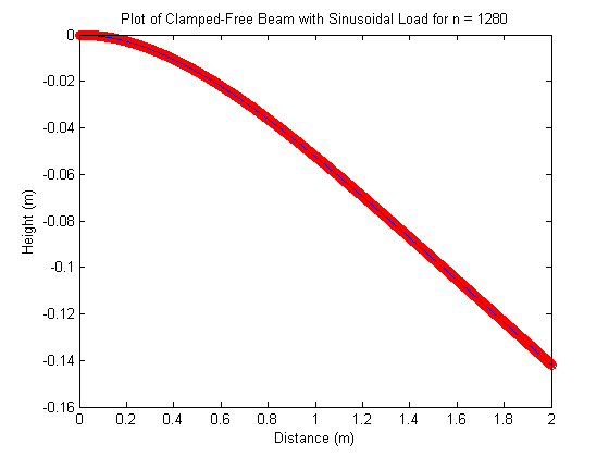
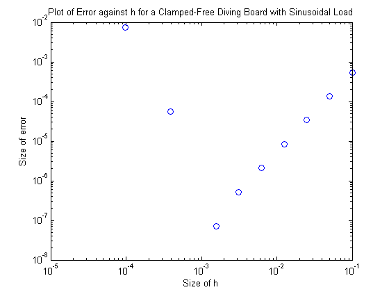
5. Rerun the calculation as in Step 3 for the sinusoidal load. (Be sure to include the weight of the beam itself.) Set \(p=100 \frac{kg}{m}\) and plot your computed solutions against the correct solution. Answer the questions from Step 3, and in addition the following one: Is the error at \(x=L\) proportional to \(h^2\) as claimed above? You may want to plot the error versus \(h\) on a log-log graph to investigate this question. Does the condition number come into play? Figure 5.2 displays the plot produced (for error vs. h) and it appears to have a constant slope. In the plot, the error of the plot at each interval size h was plotted on a log-log scale. What may be observed is that on the log-log scale, a linear plot exists. To establish the slope of this line, we take the error for \(n = 20\) and \(n = 40\), denoted \(y_{20}\) and \(y_{40}\) respectively, and the h size for \(n = 20\) and \(n = 40\), denoted \(h_{20}\) and \(h_{40}\). We will approximate our slope as \(m = \frac{log(y_{40}) - log(y_{20})}{log(h_{40}) - log(h_{20})}\). This value came out as \( m = 1.988871933346928 \approx 2\). What this describes is that for \(error = y(h)\) on our log-log scale we detect a function of \( y = mh + b\). Here, \(b\) is the y-intercept, and \(m\) the slope. As we have established the slope to be approximately 2, and our values have had their log taken, the function is more accurately represented by, \(log(y) = mlog(h) + log(c)\), where \(b = log(c)\). Thus our function is truly \( y = ch^m\). As \(m = 2\), this is \(y = ch^2\) and thus our error is indeed proportional to \(h^2\). Figure (5.1) 
Click on picture to view the associated code. Figure (5.2) 
Click on picture to view the associated code.
|