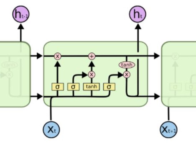
This is the course project for Statistical learning course I took in GMU. I explore how to use recurrent neural network for sequential data modeling, specific using Long Short-Term Memory (LSTM) networks to make stock market predictions. This LSTM model was inspirded by the following post Stock Market Predictions with LSTM in Python. The plot in this post can be found in Colah's blog. Colah did great job for explaining LSTM. Check out his blog Understanding LSTM Networks for more details about LSTM.
Import module first
from yahoofinancials import YahooFinancials
import numpy as np
import matplotlib.pyplot as plt
import datetime as dt
import pandas as pd
from sklearn.preprocessing import MinMaxScaler
from keras.models import Sequential
from keras.layers import Dense
from keras.layers import LSTM
from keras.layers import Dropout
Using TensorFlow backend.Read Stock Price Data from Yahoo Finance
yahoo_financials = YahooFinancials('TSLA')
stock = yahoo_financials.get_historical_price_data("2012-01-01", "2019-05-01", "daily")['TSLA']
data = pd.DataFrame(stock['prices']).iloc[:, [1,3,4,5,6]]
data.formatted_date = pd.to_datetime(data.formatted_date)
data = data.set_index('formatted_date')
data.tail()| close | high | low | open | |
|---|---|---|---|---|
| formatted_date | ||||
| 2019-04-24 | 258.660004 | 265.320007 | 258.000000 | 263.850006 |
| 2019-04-25 | 247.630005 | 259.000000 | 246.070007 | 255.000000 |
| 2019-04-26 | 235.139999 | 246.679993 | 231.130005 | 246.500000 |
| 2019-04-29 | 241.470001 | 243.979996 | 232.169998 | 235.860001 |
| 2019-04-30 | 238.690002 | 244.210007 | 237.000000 | 242.059998 |
Plot open, close, low, high stock prices
The reason I picked tesla is that this graph is bursting with different behaviors of stock prices over time. This will make the learning more robust as well as give you a change to test how good the predictions are for a variety of situations.
Another thing to notice is that the values close to 2018 are much higher and fluctuate more than the values close to the 2012. Therefore you need to make sure that the data behaves in similar value ranges throughout the time frame. You will take care of this during the data normalization phase.
plt.figure(figsize = (18,9))
plt.plot(data["open"])
plt.plot(data["high"])
plt.plot(data["low"])
plt.plot(data["close"])
plt.title('Tesla stock price history')
plt.ylabel('Price (USD)')
plt.xlabel('Days')
plt.legend(['Open','High','Low','Close'], loc='upper left')
plt.show()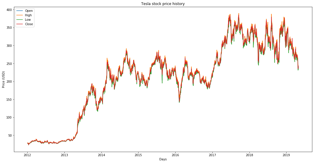
It seems the prices —Open, Close, Low, High — don’t vary too much from each other except for occasional slight drops in Low price. For simplicity, we use close price to respesent stock price on that day.
data = data["close"]Check Null/Nan Values in our data
print("checking if any null values are present\n", data.isna().sum())checking if any null values are present
0Splitting Data into a Training set and a Test set
train =  data[ : "2019-01-01"]
test = data["2019-01-01" : ]
test.head()
formatted_date
2019-01-02 310.119995
2019-01-03 300.359985
2019-01-04 317.690002
2019-01-07 334.959991
2019-01-08 335.350006
Name: close, dtype: float64One-Step Ahead Prediction via Simple Moving Average(SMA)
The prediction at t+1 is the average value of all the stock prices you observed within a window of t to t−N.
\[\large \hat{X}_{t+1} = \frac{1}{N}\sum_{i=t-N}^{t}X_{i}\]
We are going to predict the ckose stock price of the data based on the close stock prices for the past 60 days.
window_size = 60
data1 = data[train.size - window_size : data.size]
N = data1.size
std_avg_predictions = []

for pred_idx in range(window_size,N):
    std_avg_predictions.append(np.mean(data1[pred_idx-window_size:pred_idx]))


print('MSE error for SMA: %.5f'%(0.5*np.mean((std_avg_predictions - test)**2)))

plt.figure(figsize = (18,9))
plt.plot(range(window_size,N),test,color='b',label='True')
plt.plot(range(window_size,N),std_avg_predictions,color='orange',label='Prediction')
plt.xlabel('Date')
plt.ylabel('Close Stock Price(USD)')
plt.legend(fontsize=18)
plt.show()
MSE error for SMA: 417.30120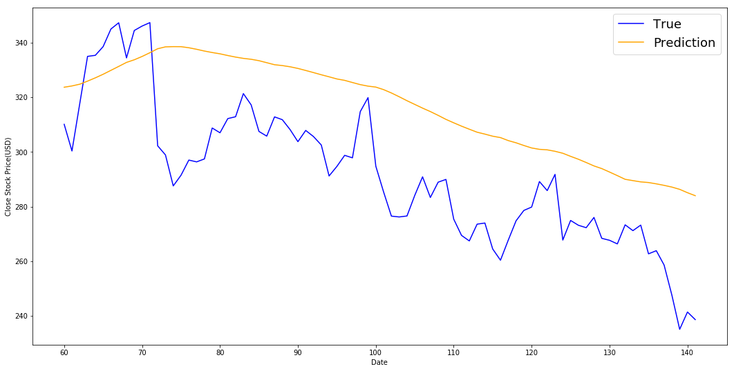
Given that stock prices don't change from 0 to 100 overnight, prediction only capture the trend of this series while the variation information is completely missing. So this result is not satisfying.
One-Step Ahead Prediction via Exponential Moving Average(EMA)
\[ \large \hat{X}_{t+1} = \text{EMA}_{t} = \gamma \times \text{EMA}_{t-1} + (1 - \gamma)X_{t} \]
The exponential moving average from t+1 time step and uses that as the one step ahead prediction. γ decides what the contribution of the most recent prediction is to the EMA, where $\text{EMA}_{0} = 0$.
exp_avg_predictions = []

running_mean = 0.0
exp_avg_predictions.append(running_mean)

decay = 0.5

for pred_idx in range(1,N):

    running_mean = running_mean*decay + (1.0-decay)*data1[pred_idx-1]
    exp_avg_predictions.append(running_mean)

plt.figure(figsize = (18,9))
plt.plot(range(window_size,N),test,color='b',label='True')
plt.plot(range(window_size,N),std_avg_predictions,color='orange',label='Prediction(SMA)')
plt.plot(range(window_size,N),exp_avg_predictions[window_size-1:N-1],color='red',label='Prediction(EMA)')
plt.xlabel('Date')
plt.ylabel('Close Stock Price(USD)')
plt.legend(fontsize=18)
plt.show()

print('MSE error for SMA: %.5f'%(0.5*np.mean((std_avg_predictions - test)**2)))
print('MSE error for EMA averaging: %.5f'%(0.5*np.mean((exp_avg_predictions[window_size-1:N-1] - test)**2)))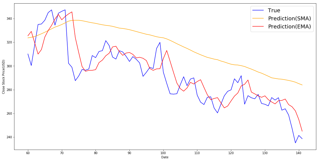
MSE error for SMA: 417.30120
MSE error for EMA averaging: 100.90856
The MSE of EMA is much lower than SMA, and EMA fits true times series pretty well in the sense that it capture variation of the price changes.
LSTM NN
Data normalization
As a rule of thumb, whenever you use a neural network, you should normalize or scale your data. We will scale our data between 0 and 1.
data2 = train.values
data2 = data2.reshape(-1,1)
scaler = MinMaxScaler(feature_range = (0, 1))
data2 = scaler.fit_transform(data2)
data2 = data2.reshape(-1)
plt.plot(data2)[] 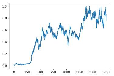
Data Preprocessing
features_set = []
labels = []
for i in range(window_size, data2.size):
    features_set.append(data2[i-window_size:i])
    labels.append(data2[i])
features_set, labels = np.array(features_set), np.array(labels)
features_set = np.reshape(features_set, (features_set.shape[0], features_set.shape[1], 1)) np.shape(features_set)(1700, 60, 1)np.shape(labels)(1700,)Training the LSTM
We need to instantiate the Sequential class. This will be our model class and we will add LSTM, Dropout and Dense layers to this model. We call the compile method on the Sequential model object which is "model" in our case. Dropout layer is added to avoid over-fitting, We use the mean squared error as loss function and to reduce the loss or to optimize the algorithm, we use the adam optimizer.
Notes: batch_size denotes the subset size of your training sample (e.g. 100 out of 1000) which is going to be used in order to train the network during its learning process. Each batch trains network in a successive order, taking into account the updated weights coming from the appliance of the previous batch.
model = Sequential()
model.add(LSTM(units=50, return_sequences=True, input_shape=(features_set.shape[1], 1)))
model.add(Dropout(0.2))
model.add(LSTM(units=50, return_sequences=True))
model.add(Dropout(0.2))
model.add(LSTM(units=50, return_sequences=True))
model.add(Dropout(0.2))
model.add(LSTM(units=50))
model.add(Dropout(0.2))
model.add(Dense(units = 1))
model.compile(optimizer = 'adam', loss = 'mean_squared_error')
model.fit(features_set, labels, epochs = 100, batch_size = 20)
WARNING:tensorflow:From D:\python\lib\site-packages\tensorflow\python\framework\op_def_library.py:263: colocate_with (from tensorflow.python.framework.ops) is deprecated and will be removed in a future version.
Instructions for updating:
Colocations handled automatically by placer.
WARNING:tensorflow:From D:\python\lib\site-packages\keras\backend\tensorflow_backend.py:3445: calling dropout (from tensorflow.python.ops.nn_ops) with keep_prob is deprecated and will be removed in a future version.
Instructions for updating:
Please use `rate` instead of `keep_prob`. Rate should be set to `rate = 1 - keep_prob`.
WARNING:tensorflow:From D:\python\lib\site-packages\tensorflow\python\ops\math_ops.py:3066: to_int32 (from tensorflow.python.ops.math_ops) is deprecated and will be removed in a future version.
Instructions for updating:
Use tf.cast instead.
Epoch 1/100
1700/1700 [==============================] - 17s 10ms/step - loss: 0.0252
Epoch 2/100
1700/1700 [==============================] - 12s 7ms/step - loss: 0.0071
Epoch 3/100
1700/1700 [==============================] - 12s 7ms/step - loss: 0.0064
Epoch 4/100
1700/1700 [==============================] - 12s 7ms/step - loss: 0.0053
Epoch 5/100
1700/1700 [==============================] - 12s 7ms/step - loss: 0.0057
Epoch 6/100
1700/1700 [==============================] - 12s 7ms/step - loss: 0.0051
Epoch 7/100
1700/1700 [==============================] - 12s 7ms/step - loss: 0.0053
Epoch 8/100
1700/1700 [==============================] - 12s 7ms/step - loss: 0.0052
Epoch 9/100
1700/1700 [==============================] - 12s 7ms/step - loss: 0.0042
Epoch 10/100
1700/1700 [==============================] - 12s 7ms/step - loss: 0.0041
Epoch 11/100
1700/1700 [==============================] - 12s 7ms/step - loss: 0.0038
Epoch 12/100
1700/1700 [==============================] - 12s 7ms/step - loss: 0.0039
Epoch 13/100
1700/1700 [==============================] - 12s 7ms/step - loss: 0.0038
Epoch 14/100
1700/1700 [==============================] - 12s 7ms/step - loss: 0.0038
Epoch 15/100
1700/1700 [==============================] - 12s 7ms/step - loss: 0.0033
Epoch 16/100
1700/1700 [==============================] - 12s 7ms/step - loss: 0.0032
Epoch 17/100
1700/1700 [==============================] - 12s 7ms/step - loss: 0.0031
Epoch 18/100
1700/1700 [==============================] - 12s 7ms/step - loss: 0.0031
Epoch 19/100
1700/1700 [==============================] - 12s 7ms/step - loss: 0.0032
Epoch 20/100
1700/1700 [==============================] - 12s 7ms/step - loss: 0.0030
Epoch 21/100
1700/1700 [==============================] - 12s 7ms/step - loss: 0.0029
Epoch 22/100
1700/1700 [==============================] - 12s 7ms/step - loss: 0.0026
Epoch 23/100
1700/1700 [==============================] - 12s 7ms/step - loss: 0.0029
Epoch 24/100
1700/1700 [==============================] - 12s 7ms/step - loss: 0.0026
Epoch 25/100
1700/1700 [==============================] - 13s 7ms/step - loss: 0.0025
Epoch 26/100
1700/1700 [==============================] - 12s 7ms/step - loss: 0.0026
Epoch 27/100
1700/1700 [==============================] - 12s 7ms/step - loss: 0.0023
Epoch 28/100
1700/1700 [==============================] - 12s 7ms/step - loss: 0.0025
Epoch 29/100
1700/1700 [==============================] - 12s 7ms/step - loss: 0.0022
Epoch 30/100
1700/1700 [==============================] - 12s 7ms/step - loss: 0.0022
Epoch 31/100
1700/1700 [==============================] - 12s 7ms/step - loss: 0.0022
Epoch 32/100
1700/1700 [==============================] - 13s 7ms/step - loss: 0.0021
Epoch 33/100
1700/1700 [==============================] - 13s 8ms/step - loss: 0.0021
Epoch 34/100
1700/1700 [==============================] - 12s 7ms/step - loss: 0.0021
Epoch 35/100
1700/1700 [==============================] - 12s 7ms/step - loss: 0.0020
Epoch 36/100
1700/1700 [==============================] - 12s 7ms/step - loss: 0.0020
Epoch 37/100
1700/1700 [==============================] - 12s 7ms/step - loss: 0.0020
Epoch 38/100
1700/1700 [==============================] - 12s 7ms/step - loss: 0.0020
Epoch 39/100
1700/1700 [==============================] - 12s 7ms/step - loss: 0.0019
Epoch 40/100
1700/1700 [==============================] - 12s 7ms/step - loss: 0.0017
Epoch 41/100
1700/1700 [==============================] - 12s 7ms/step - loss: 0.0018
Epoch 42/100
1700/1700 [==============================] - 12s 7ms/step - loss: 0.0017
Epoch 43/100
1700/1700 [==============================] - 12s 7ms/step - loss: 0.0017
Epoch 44/100
1700/1700 [==============================] - 12s 7ms/step - loss: 0.0018
Epoch 45/100
1700/1700 [==============================] - 12s 7ms/step - loss: 0.0017
Epoch 46/100
1700/1700 [==============================] - 12s 7ms/step - loss: 0.0017
Epoch 47/100
1700/1700 [==============================] - 12s 7ms/step - loss: 0.0018
Epoch 48/100
1700/1700 [==============================] - 12s 7ms/step - loss: 0.0019
Epoch 49/100
1700/1700 [==============================] - 12s 7ms/step - loss: 0.0018
Epoch 50/100
1700/1700 [==============================] - 12s 7ms/step - loss: 0.0015
Epoch 51/100
1700/1700 [==============================] - 12s 7ms/step - loss: 0.0015
Epoch 52/100
1700/1700 [==============================] - 12s 7ms/step - loss: 0.0015
Epoch 53/100
1700/1700 [==============================] - 12s 7ms/step - loss: 0.0016
Epoch 54/100
1700/1700 [==============================] - 12s 7ms/step - loss: 0.0015
Epoch 55/100
1700/1700 [==============================] - 12s 7ms/step - loss: 0.0015
Epoch 56/100
1700/1700 [==============================] - 12s 7ms/step - loss: 0.0015
Epoch 57/100
1700/1700 [==============================] - 12s 7ms/step - loss: 0.0015
Epoch 58/100
1700/1700 [==============================] - 12s 7ms/step - loss: 0.0013
Epoch 59/100
1700/1700 [==============================] - 12s 7ms/step - loss: 0.0014
Epoch 60/100
1700/1700 [==============================] - 12s 7ms/step - loss: 0.0014
Epoch 61/100
1700/1700 [==============================] - 12s 7ms/step - loss: 0.0013
Epoch 62/100
1700/1700 [==============================] - 12s 7ms/step - loss: 0.0014
Epoch 63/100
1700/1700 [==============================] - 12s 7ms/step - loss: 0.0014
Epoch 64/100
1700/1700 [==============================] - 13s 7ms/step - loss: 0.0015
Epoch 65/100
1700/1700 [==============================] - 12s 7ms/step - loss: 0.0014
Epoch 66/100
1700/1700 [==============================] - 12s 7ms/step - loss: 0.0012
Epoch 67/100
1700/1700 [==============================] - 12s 7ms/step - loss: 0.0014
Epoch 68/100
1700/1700 [==============================] - 12s 7ms/step - loss: 0.0012
Epoch 69/100
1700/1700 [==============================] - 12s 7ms/step - loss: 0.0013
Epoch 70/100
1700/1700 [==============================] - 12s 7ms/step - loss: 0.0013
Epoch 71/100
1700/1700 [==============================] - 12s 7ms/step - loss: 0.0014
Epoch 72/100
1700/1700 [==============================] - 12s 7ms/step - loss: 0.0013
Epoch 73/100
1700/1700 [==============================] - 13s 7ms/step - loss: 0.0014
Epoch 74/100
1700/1700 [==============================] - 12s 7ms/step - loss: 0.0014
Epoch 75/100
1700/1700 [==============================] - 12s 7ms/step - loss: 0.0013
Epoch 76/100
1700/1700 [==============================] - 12s 7ms/step - loss: 0.0013
Epoch 77/100
1700/1700 [==============================] - 12s 7ms/step - loss: 0.0014
Epoch 78/100
1700/1700 [==============================] - 12s 7ms/step - loss: 0.0013
Epoch 79/100
1700/1700 [==============================] - 12s 7ms/step - loss: 0.0012
Epoch 80/100
1700/1700 [==============================] - 12s 7ms/step - loss: 0.0012
Epoch 81/100
1700/1700 [==============================] - 12s 7ms/step - loss: 0.0012
Epoch 82/100
1700/1700 [==============================] - 13s 7ms/step - loss: 0.0010
Epoch 83/100
1700/1700 [==============================] - 12s 7ms/step - loss: 0.0011
Epoch 84/100
1700/1700 [==============================] - 12s 7ms/step - loss: 0.0012
Epoch 85/100
1700/1700 [==============================] - 12s 7ms/step - loss: 0.0013
Epoch 86/100
1700/1700 [==============================] - 12s 7ms/step - loss: 0.0012
Epoch 87/100
1700/1700 [==============================] - 12s 7ms/step - loss: 0.0012
Epoch 88/100
1700/1700 [==============================] - 12s 7ms/step - loss: 0.0012
Epoch 89/100
1700/1700 [==============================] - 12s 7ms/step - loss: 0.0012
Epoch 90/100
1700/1700 [==============================] - 12s 7ms/step - loss: 0.0011
Epoch 91/100
1700/1700 [==============================] - 12s 7ms/step - loss: 0.0011
Epoch 92/100
1700/1700 [==============================] - 12s 7ms/step - loss: 0.0012
Epoch 93/100
1700/1700 [==============================] - 12s 7ms/step - loss: 0.0013
Epoch 94/100
1700/1700 [==============================] - 12s 7ms/step - loss: 0.0011
Epoch 95/100
1700/1700 [==============================] - 12s 7ms/step - loss: 0.0013
Epoch 96/100
1700/1700 [==============================] - 12s 7ms/step - loss: 0.0011
Epoch 97/100
1700/1700 [==============================] - 12s 7ms/step - loss: 0.0011
Epoch 98/100
1700/1700 [==============================] - 12s 7ms/step - loss: 0.0011
Epoch 99/100
1700/1700 [==============================] - 12s 7ms/step - loss: 0.0011
Epoch 100/100
1700/1700 [==============================] - 12s 7ms/step - loss: 0.0011
Testing our LSTM
test1 = data1.values
test1 = test1.reshape(-1,1)
test1 = scaler.transform(test1)
test1 = test1.reshape(-1)
test_features = []
for i in range(window_size, test1.size):
    test_features.append(test1[i-window_size:i])

test_features = np.array(test_features)
test_features = np.reshape(test_features, (test_features.shape[0], test_features.shape[1], 1))

predictions = model.predict(test_features)
predictions = scaler.inverse_transform(predictions)
predictions = predictions.reshape(-1)

plt.figure(figsize = (18,9))
plt.plot(range(window_size,N),data1[window_size-1:N-1],color='b',label='True')
plt.plot(range(window_size,N),std_avg_predictions,color='orange',label='Prediction(SMA)')
plt.plot(range(window_size,N),exp_avg_predictions[window_size-1:N-1],color='red',label='Prediction(EMA)')
plt.plot(range(window_size,N),predictions,color='green',label='Prediction(LSTM)')
plt.xlabel('Date')
plt.ylabel('Close Stock Price(USD)')
plt.legend(fontsize=18)
plt.show()

print('MSE error for SMA: %.5f'%(0.5*np.mean((std_avg_predictions - test)**2)))
print('MSE error for EMA averaging: %.5f'%(0.5*np.mean((exp_avg_predictions[window_size-1:N-1] - test)**2)))
print('MSE error for LSTM: %.5f'%(0.5*np.mean((predictions - test)**2)))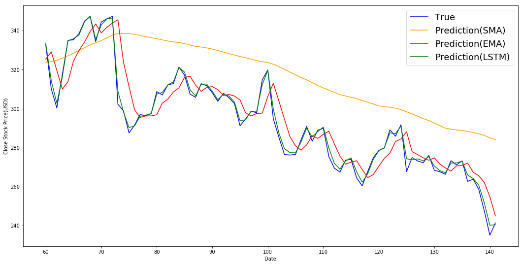
MSE error for SMA: 417.30120
MSE error for EMA averaging: 100.90856
MSE error for LSTM: 48.48832
Multi-Step Ahead Prediction via Exponential Moving Average(EMA)
Since you can't do much with just the stock market value of the next day, we would like to know the stock market prices go up or down in the next four months. However no matter how many steps you predict in to the future, you'll keep getting the same answer for all the future prediction steps for EMA.
To see this, Consider \(\hat{X}_{t+1} = \text{EMA}_{t} , \hat{X}_{t+2} = \gamma \times \hat{X}_{t+1} + (1 - \gamma) \times \text{EMA}_{t} = \gamma \times \hat{X}_{t+1} + (1 - \gamma) \times \hat{X}_{t+1} = \hat{X}_{t+1}\)
Multi-Step Ahead Prediction via LSTM
Long Short-Term Memory models are extremely powerful time-series models. They can predict an arbitrary number of steps into the future. I am trying to apply multiple LSTM on Tesla.
Peace!