Yasin Hassan Project 3

We are tying to plot the data of coronavirus. We set T=[1:17] and Y=[9;6;15;10;16;10;18;18;29;28;14;13;4;31;27;30;52].

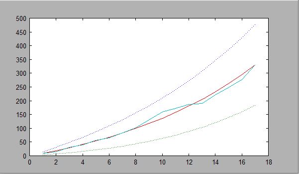
For problem 1 with the least square fit,a should be [2,12;0.072], and I got a=[2.12376191853455;0.07270359879536] so my value is accurate

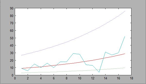
For problem 2, I plotted the least squares fit. We did upper = exp(a(1)+a(2)*T+2*stddev); middle = exp(a(1)+a(2)*T); lower = exp(a(1)+a(2)*T-2*stddev);

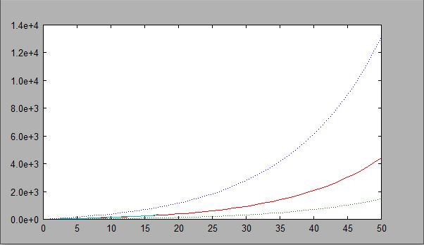
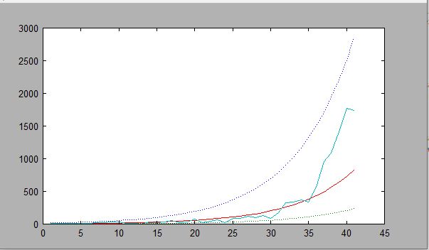
For problem 3, I plotted the cumulative sum. The original values only go up to 17, but this graph predicts the line up to T=50. The is what the graph looked like.

For problem 4, gradient of L, DL=[-exp(a(1)+a(2)*i)+Y(i);-i*exp(a(1)+a(2)*i)+i*Y(i)]

For problem 5 we need to fing the hessian, LH. LH = [-exp(a(1)+a(2)*i) -i*exp(a(1)+a(2)*i);-i*exp(a(1)+a(2)*i) -(i^2)*exp(a(1)+a(2)*i)];

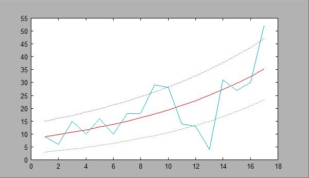
For problem 6, we used Newton's method, a0 = a0 - LH\DL, where a0=[2.12;0.07] as the initial guess. I got a0= [2.11380701774804; 0.08516747146626].

For problem 7, we did upper1 = exp(a0(1)+a0(2)*T)+2*sqrt(exp(a0(1)+a0(2)*T)); lower1 = exp(a0(1)+a0(2)*T)-2*sqrt(exp(a0(1)+a0(2)*T)); middle1 = exp(a0(1)+a0(2)*T);

First, we did the least squares fit.

Then, we did the cumulative sum.

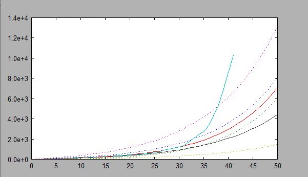
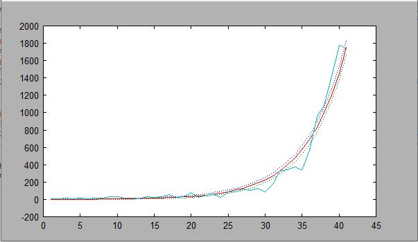
For Problem 8, we changed the T=[1:50] and we set Y2=[9,15,30,40,56,66,84,102,131,159,173,186,190,221,248,278,330,354,382,461,481,526,587,608,697,781,896,999,1124,1212,1385,1715,2055,2429,2764,3332,4288,5373,6789,8564,10298]'; and T2 = [1:length(Y2)];. We plotted the least squares(black), poissin(red) and the true value(blue). You can see that they're equal to each other until T=20. The poisson and true value are equal until T=32.

For problem 9, whe changed T=[1:200]; and Y=[9,15,30,40,56,66,84,102,131,159,173,186,190,221,248,278,330,354,382,461,481,526,587,608,697,781,896,999,1124,1212,1385,1715,2055,2429,2764,3332,4288,5373,6789,8564,10298]';

We got a = [1.47941170509351;0.12766927914537], DL = 1.0e+005 *[0.03461878663866;1.40515373856399]. After doing Newton's method, we get a0 =[-0.16566281309009;0.18617403527988].

For the least squares fit, we get

for the poisson

I changes the values, and upper1 = exp(a0(1)+a0(2)*T)+2*sqrt(exp(a0(1)+a0(2)*T)); lower1 = exp(a0(1)+a0(2)*T)-2*sqrt(exp(a0(1)+a0(2)*T)); middle1 = exp(a0(1)+a0(2)*T);

For the least squares.

For the poisson

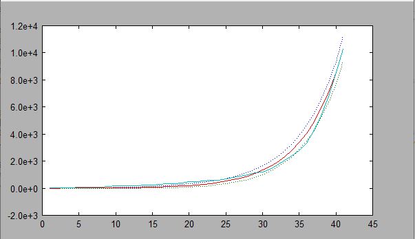
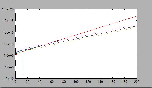
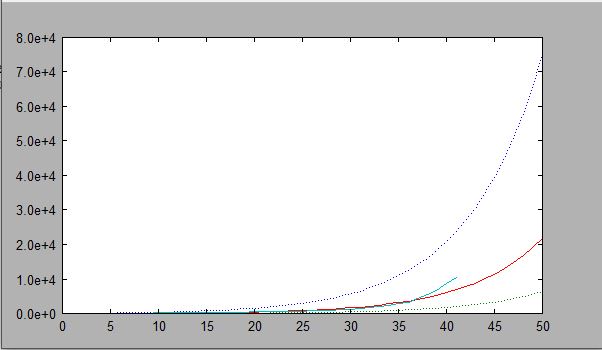
Finally, we changes the T values to T=[1:200]. I graph the least squares for the original upper, middle and lower(black), the poisson for the adjusted upper, middle, and lower(red), and the true value(light blue). As you can see, all of the values fit better. According to the Poisson value, the original plot hits Y=1,000,000 at T=62.