y = dct(x) returns the unitary discrete cosine transform of x,
![]()
where
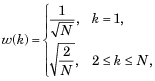
N is the length of x, and x and y are the same size. If x is a matrix, dct transforms its columns.
The two-dimenstional Discrete Cosine Transform is the one-dimensional DCT applied in the two dimnesions. In the case of JPEG format, the two-dimensional DCT is applied to 8x8 pixel blocks of the image. In our project we listed the vertical coordinate first and the horizontal coordinate second when referencing a 2-dimesnsional gridpoint. The 2D-DCT constructs an interpolating function using least squares that is then applied successively to both horizontal and vertical directions of each 8x8 block.
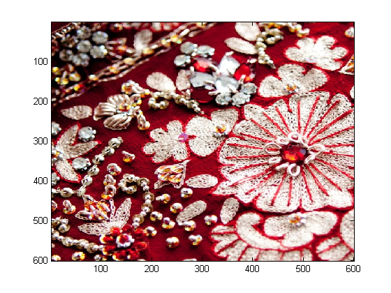
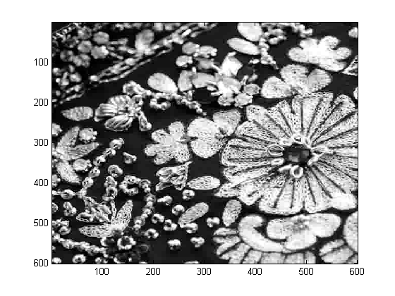
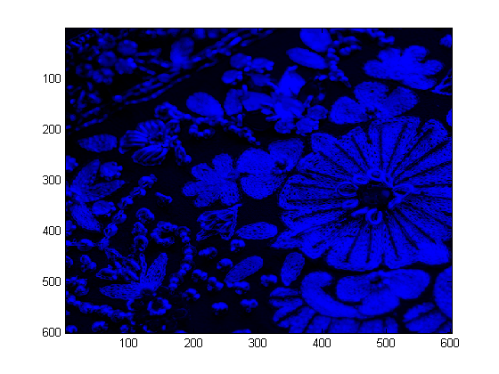
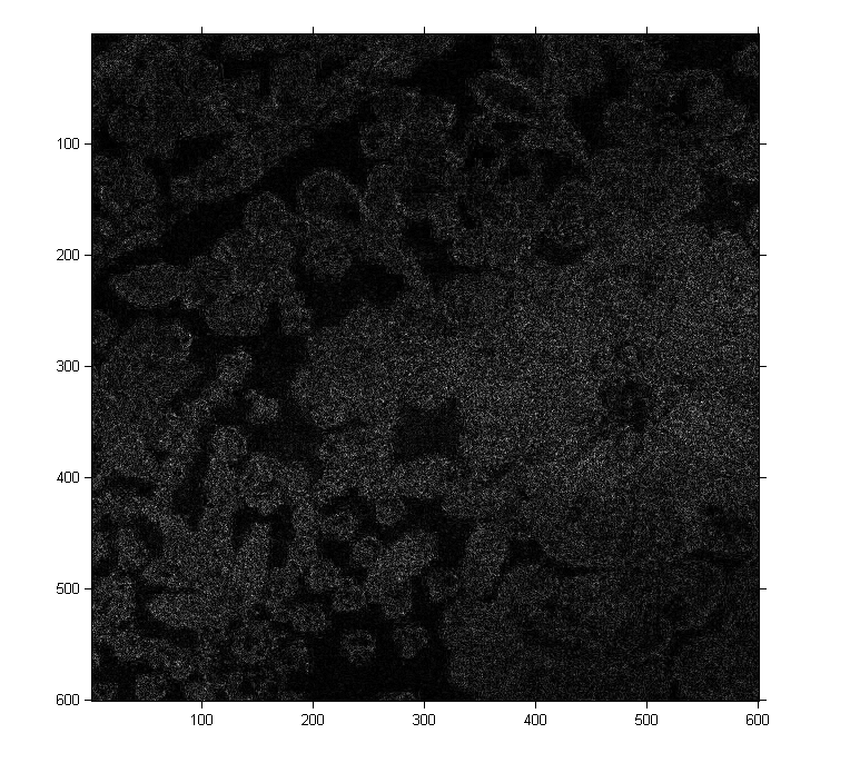
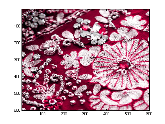
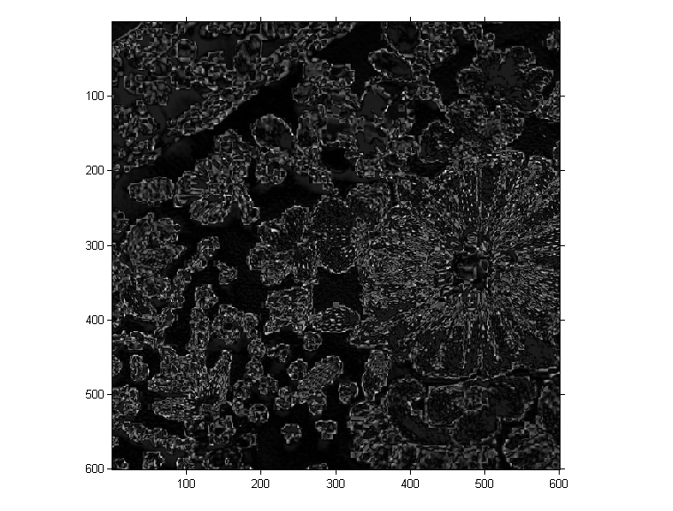
We first chose a JPEG image. The image chosen is a picture of the details of embroidery on a traditional wedding sari. We chose a 600x600 sample of the image to make traversal of the image even and converted the image to grayscale. .
 |  |
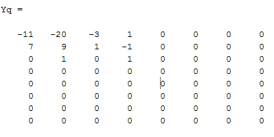
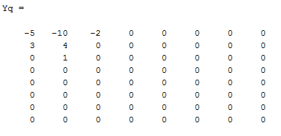
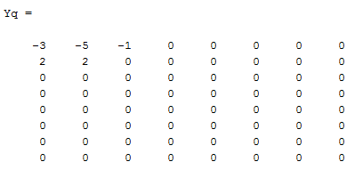
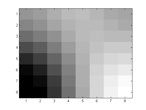
We then extracted an 8x8 pixel block from the image. We then applied the 2D-DCT and quantized using linear quantization matrix defined by Q=p*8./hilb(8), where p is the loss paramater and hilb(8) is the Hilbert matrix with denominator as multiples of 8. The following are the compressed matrices for p = 1, 2 and 4.
| Yq for p=1 | Yq for p=2 | Yq for p=4 |
 |  |  |
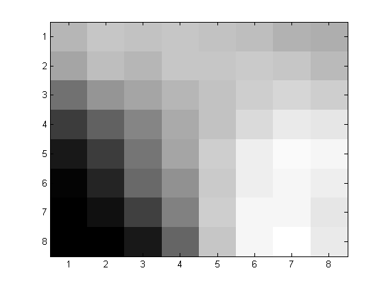
We then reconstructed the 8x8 block by using MATLAB's inverse DCT function, idct(x), and compared the new image with the original.
| Before 8x8 | After with p=1 |
 | 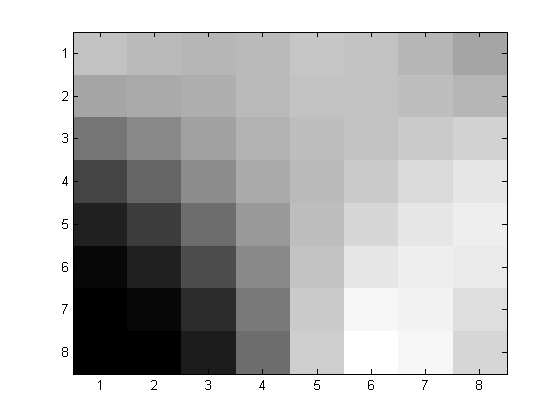 |
| Before 8x8 | After with p=2 |
| 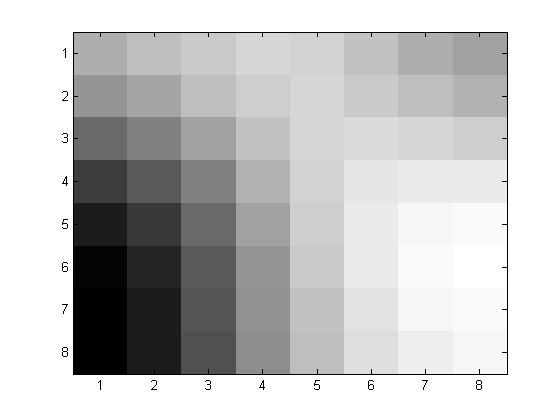 |
| Before 8x8 | After with p=4 |
|  |
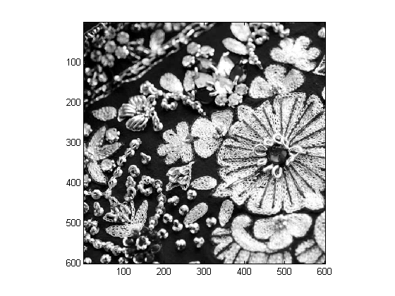
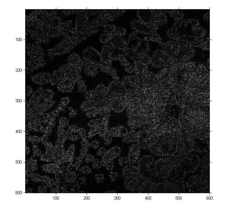
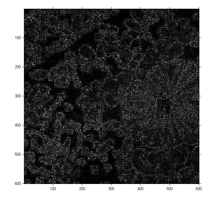
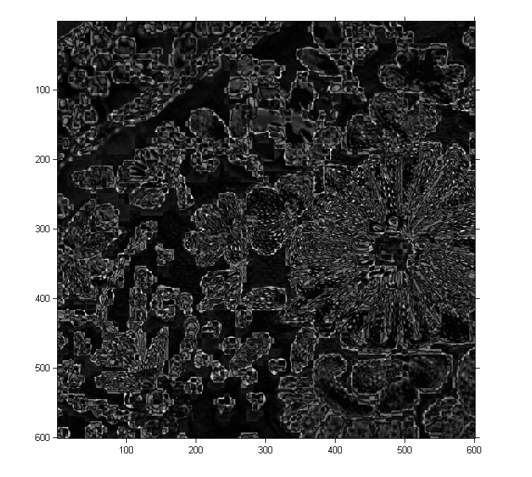
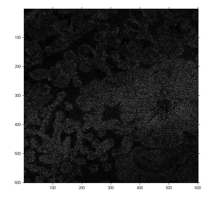
Finally, the compression and reconstitution of the image was done for all the the 8x8 blocks of the image which yielded the following results:
| Original BW | After with p=1 |
|  |
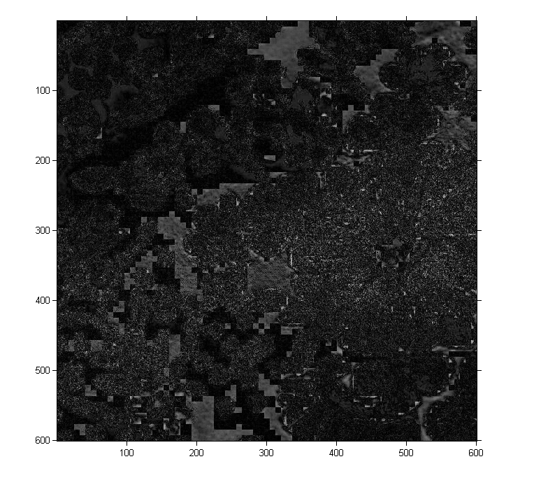
| Original BW | After with p=2 |
|  |
| Original BW | After with p=4 |
|  |
The code for the process described above can be found here.
| Original BW | JPEG-suggested Matrix with p=1 | Hilbert Matrix with p=1 |
|  | |
The code for the process described above can be found here.
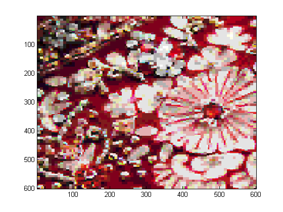
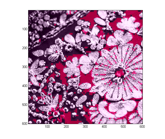
We seperated the red, blue and green from the color image and conducted compression and dequanitization seperately, then reconstituted as a color image.
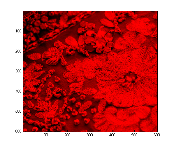 |  |  |
| Original Color | After with p=1 | Comparison |
|  |  |
| Original Color | After with p=10 | Comparison |
|  |  |
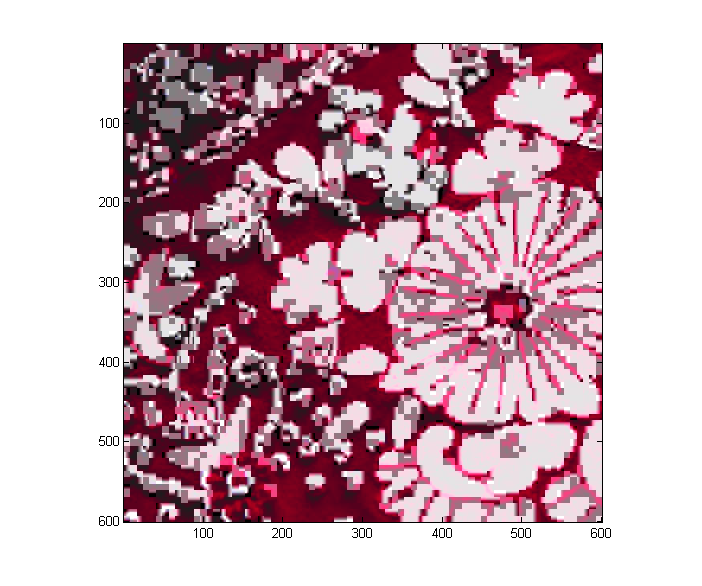
| Original Color | After with p=50 | Comparison |
|  |  |
| Original Color | After with p=100 | Comparison |
| 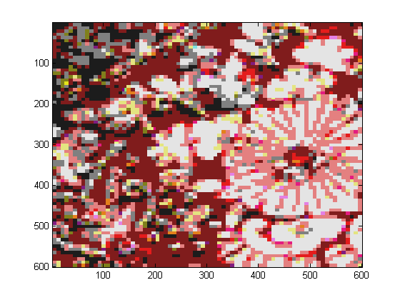 |  |
The code for the process described above can be found here.
The baseline JPEG method transforms RGB color data to the YUV system, where Y represents luminance and U, V represent color differences. After defining Y, U, and V we compressed using JPEG quantization and then reconstituted as a color image with the following results.
| Original Color | After with p=1 | Comparison |
|  |  |
| Original Color | After with p=1 | Comparison |
| | |
| YUV | QC Amped | QC AmpedComparison |
|  |  |
| YUV | QY Amped | QY AmpedComparison |
|  |  |
The code for the process described above can be found here.