
In this project, we will be modeling the steady-state distribution along a rectangular fin of a heat sink. A heat sink is a passive heat exchanger that cools a device by dissipating heat into the surrounding medium. Our main goal is then keep the temperature of the heat sink in the appropiate range by determining the dimensions of the fin. The given fin is a rectangular slab with dimensions \(L_x \times L_y\) and width \(\delta\), where \(\delta\) is relatively small.
We will consider two ways in which heat moves: conduction and convection. In conduction, heat is transmitted through collisions between neighboring molecules; while in convection, heat is transmitted due to the motion itself of the molecules.
For conduction, we use Fourier's first law: $$q = -K A \nabla u$$ where \(q\) is heat energy per unit time (in watts) \(A\) is the material's cross-sectional area, \(\nabla u\) is the gradient of the temperature, and \(K\) is the material's thermal conductivity.
For convection, we use Newton's law of cooling: $$q = -H A (u-u_b)$$ where \(H\) is the convective heat transfer coefficient and \(u_b\) is the ambient temperature, or bulk temperature.
The following illustration, borrowed from Dr. Sauer's Numerical Analysis, gives us an idea of how conduction and convection behave on the fin:
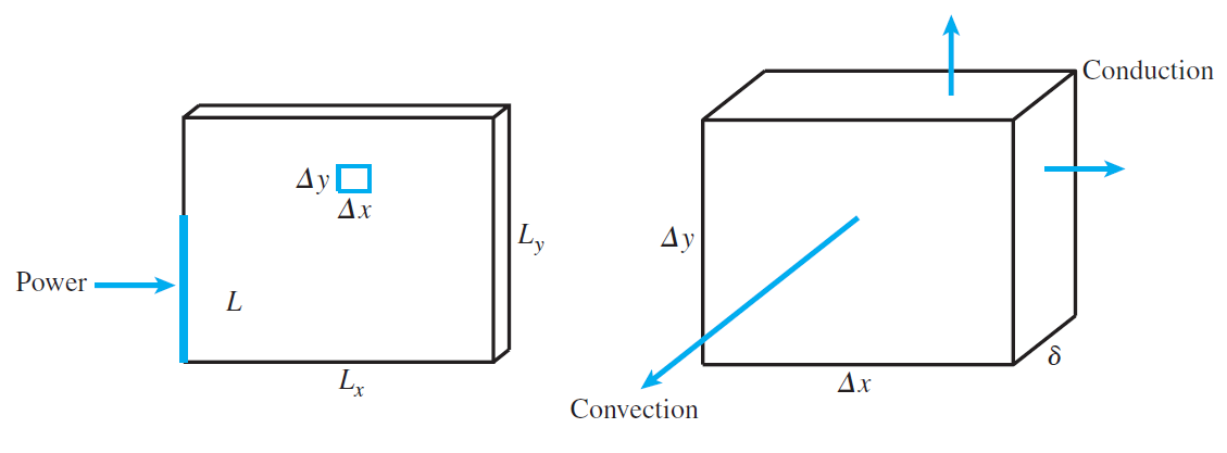
From the illustration above, we can see that heat entering the box through the two \(\Delta y \times \delta\) sides and the two \(\Delta x \times \delta\) sides is by conduction, and through the two \(\Delta x \times \Delta y\) is by convection; thus resulting in the following steady-state equation: $$-K\Delta y\delta u_x(x,y) + K\Delta y \delta u_x (x+\Delta x,y) - K\Delta x \delta u_y (x,y) + K\Delta x \delta u_y (x,y+\Delta y) - H\Delta x \Delta y u(x,y) = 0 $$
We divide by \(\Delta x \Delta y\) to obtain the following equation: $$K \delta \frac{u_x (x+\Delta x,y) - u_x (x,y)}{\Delta x} + K \delta \frac{u_y (x,y+\Delta y) - u_y (x,y)}{\Delta y} = 2Hu(x,y)$$
We look at the limit as \(\Delta x, \Delta y \rightarrow 0 \) to obtain the elliptic partial differential equation: $$u_{xx} + u_{yy} = \frac{2H}{K\delta} u$$
From this equation, we can use the following in the finite difference method to approximate \(u\) at its interior points: $$\frac{u_{i+1,j} - 2u_{i,j} + u_{i-1,j}}{h^2} + \frac{u_{i,j+1} - 2u_{i,j} + u_{i,j-1}}{k^2} = \frac{2H}{K\delta}$$ For the boundary conditions, part or all of an edge will have power surging through it, which we will use Fourier's law, \(u_{\text{normal}} = \frac{P}{L\delta K},\) to model. Using the following approximation for the first derivative $$f'(x) = \frac{-3f(x) + 4f(x + h) + f(x + 2h)}{2h} + \mathcal{O}(h^2)$$ we derive the following equation with power surging through the left edge. $$\frac{-3u_{1,j} + 4u_{2,j} - u_{3,j}}{2h} = -\frac{P}{L \delta K}$$ For the rest of the boundary points without power, we use the convective boundary condition \(Ku_{\text{normal}} = Hu\) and the above first-derivated approximation to get the following for the edges: $$\frac{-3u_{i,1} + 4u_{i,2} - u_{i,3}}{2k} = -\frac{H}{K}u_{i,1}$$ $$\frac{-3u_{i,n} + 4u_{i,n-1} - u_{i,n-2}}{2k} = -\frac{H}{K}u_{i,n}$$ $$\frac{-3u_{1,j} + 4u_{2,j} - u_{3,j}}{2h} = -\frac{H}{K}u_{1,j}$$ $$\frac{-3u_{m,j} + 4u_{m-1,j} - u_{m-2,j}}{2h} = -\frac{H}{K}u_{m,j}$$
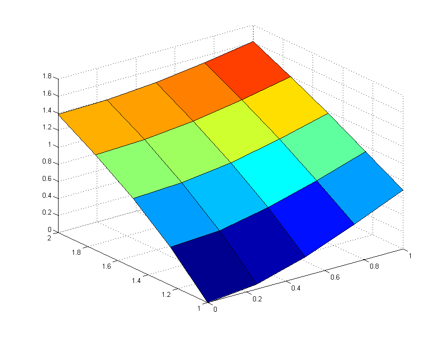
We begin by reproducing the results of Example 8.8 from our book, using poisson.m. Note that, through the project, we replace mesh with surf for a more aesthetically pleasing plot.
For problems 1-3, we will assume that our fin is composed of aluminum, whose thermal conductivity is \(K = 1.68\) W/cm\(\circ\)C. We also assume the the convective heat transfer coeffiecient is \(H = 0.005\) W/\(\text{cm}^2\)\(\circ\)C and the ambient temperature is \(u_b = 20^\circ\text{C}\).
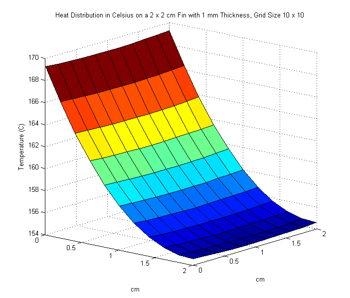
We begin with a fin of dimensions \(2 \times 2\) cm and thickness of \(1\) mm. An input power of \(5\) watts enters along the left side of the fin. We solve the ellliptic partial differential equation: $$u_{xx} + u_{yy} = \frac{2H}{K\delta} u$$ with \(M = N = 10\) steps in the \(x\) and \(y\) direction. The surf command is used to plot the resulting heat distribution over the \(xy\)-plane. We are also asked to find out what the maximum temperature of the fin is in \(^\circ\text{C}\).
We modify the original poisson code from Example 8.8 by modifying the code used to generate the matrix and vector to match the partial differential equation in the interior, as well as the equations for the points on the edges of the grid to match the Robin Boundary Conditions, and end up with poisson1.m. Running our code results in the following plot, with a maximum temperature of approximately \(169.26^\circ\text{C}\).
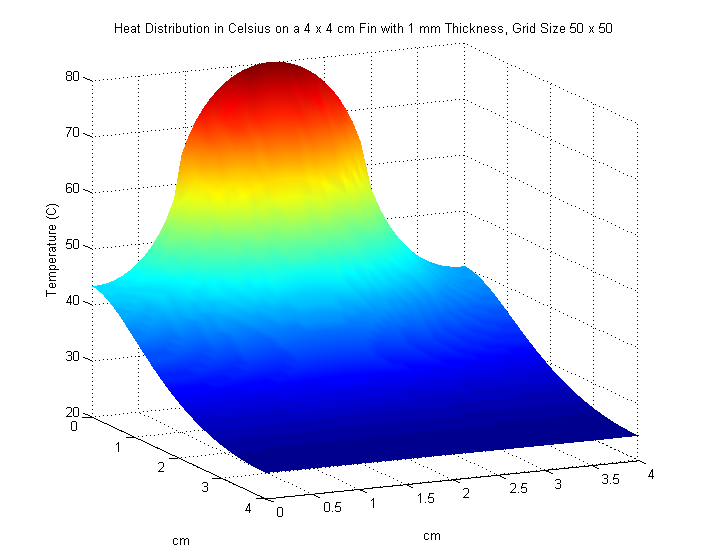
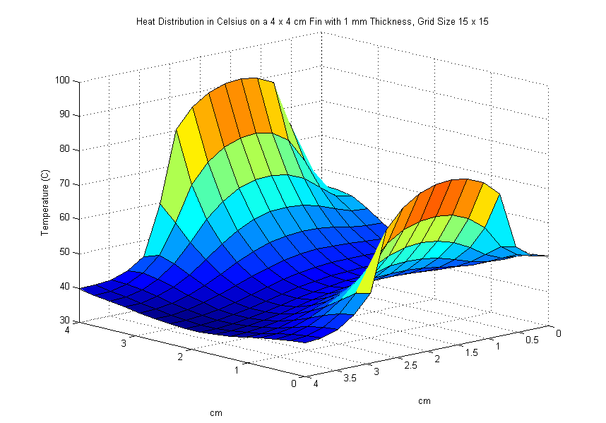
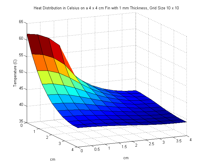
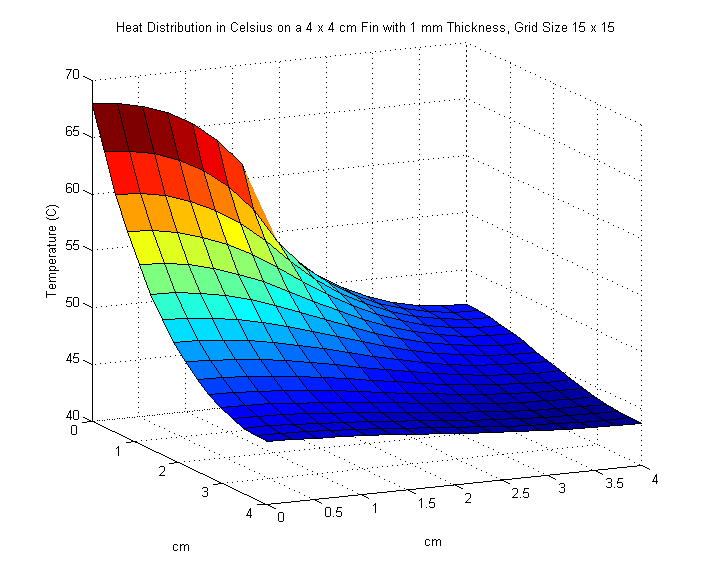
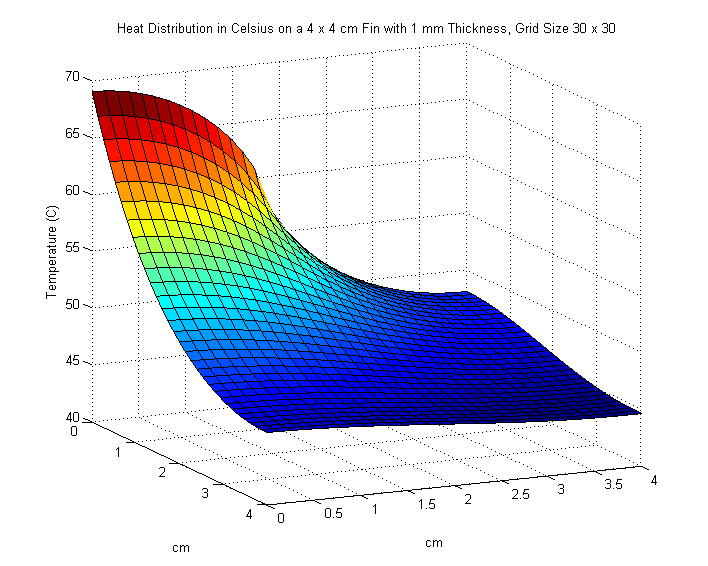
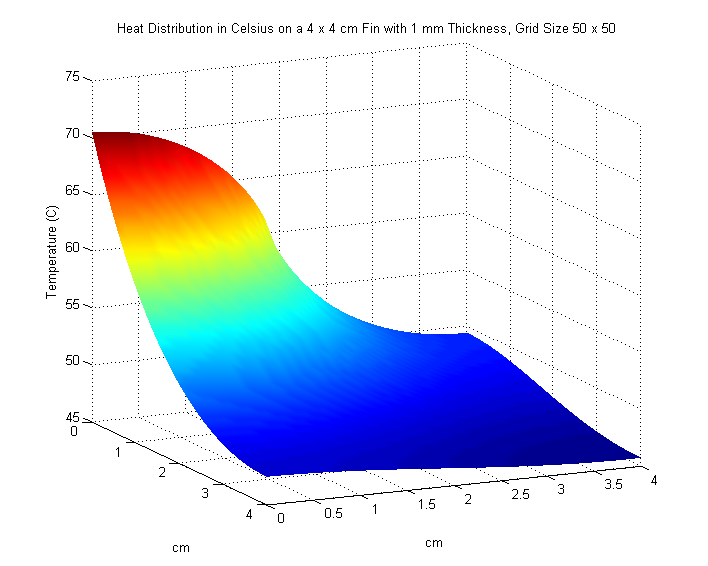
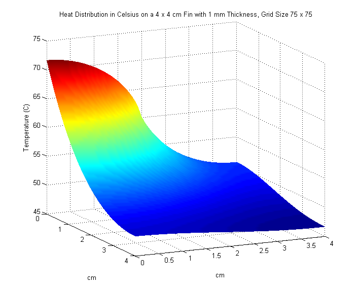
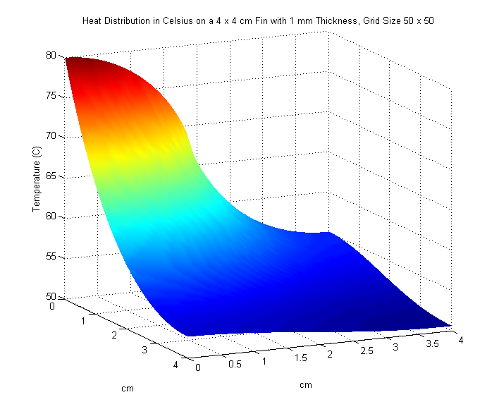
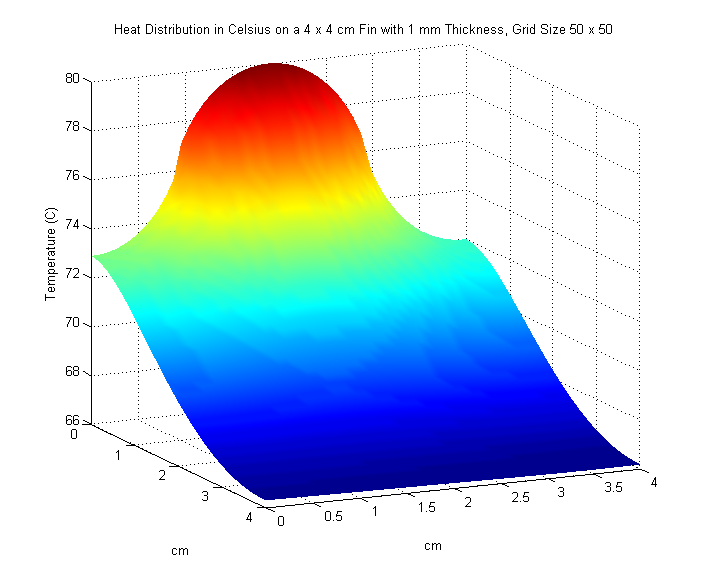
We increase the size of the fin to \(4 \times 4\) cm. An input power of \(5\) watts on the interval \([0,2]\) enters along the left side of the fin. Once again, we are asked to plot our results and find the maximum temperature of the fin in \(^\circ\text{C}\). We also experiment with different values of \(M\) and \(N\) to see any noticeable changes in our solution.
We use poisson2.m and try the following values for \(M\) and \(N\):
|
|
|
|
|
|
|
|
|
We are asked to find the maximum power that can be dissipated by a \(4 \times 4\) cm fin while maintaining the maximum temperature below \(80\) \(\circ\)C. We will assume a bulk temperature of \(20\)\(\circ\)C and an input power along \(2\) cm.
In order to find the maximum power, the bisecion method is applied in PoissonBisect.m along with poisson3.m. We obtain a value of \(5.94464060\) W for our maximum power on the interval \([0,2]\). However, changing the interval to \([1,3]\) results in a higher maximum power of \(6.32480008\) W.
|

|
We replace our aluminum fin with a copper fin, which has a thermal conductivity of \(k = 3.85 \frac{W}{cm}^\circ\text{C}\). We are asked to find the maximum power that can be dissipated by a \(4 \times 4 \text{ cm}\) fin with the \(2 \text{cm}\) power input in the optimal placement while, once again, maintaining the maximum temperature below \(80^\circ\text{C}\).
After playing with different intervals, we notice that the interval \([1,2]\) offers the most optimal placement, generating a maximum power of \(7.57206930\) W. For our results, we once again apply the bisection method with PoissonBisectCopper.m along with poisson4.m
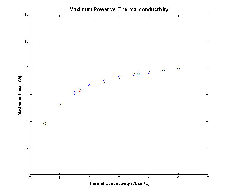
We are to plot the maximum power that can dissipated in step 4 as a function of thermal conductivity, where \(1\frac{W}{\text{cm}}^\circ\text{C}\leq K \leq 5 \frac{W}{\text{cm}}^\circ\text{C}\)
Here, we simply keep track of the maximum powers corresponding to their respective thermal conductivities. We use Plot5.m for the following plot:
We redo step 4 for a water-cooled fin. We assume that water has a convective heat transfer coeffiecient \(H = 0.1 \frac{W}{\text{cm}^2}^\circ\text{C}\) and the ambient temperature is \(u_b = 20^\circ\text{C}\).
Once again, we apply the bisection method to find the maximum power. Using PoissonBisectWater.m along with poisson6.m, we obtain a maximum power of \(36.14960773 \text{ W}\).