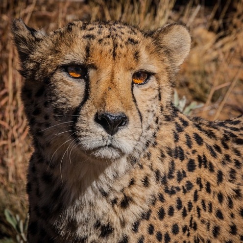
In this project, we will delve into image compression. We often have images of large size which can be difficult to manipulate or use without the right machinery. Therefore, we want to reduce the size of the image, or compress it, by performing the methods of Discrete Cosine Transform (DCT) and Quantization.
For our case, we will be using the two-dimensional Discrete Cosine Transform, which is essentially the DCT applied in two dimensions, and defined as: For a \(n \times n\) matrix \(X\), the 2D-DCT is the matrix \( Y = C X C^{T}\), where \(C\) is defined as: $$C_{ij} = \frac{\sqrt 2}{\sqrt n} a_{i} \text{cos} \frac{i(2j+1)\pi}{2n}$$ for \(i,j=0,...,n-1\), where $$a_{i} \equiv \begin{cases} \frac{1}{\sqrt 2}, & \mbox{if } \mbox{ i=0,} \\ 1, & \mbox{if } \mbox{ i=1,...,n-1} \end{cases}$$ or $$C = \sqrt{\frac{2}{n}}\left[\begin{matrix} \frac{1}{\sqrt2} & \frac{1}{\sqrt2} & \cdots & \frac{1}{\sqrt2} \\ \text{cos}\frac{\pi}{2n} & \text{cos}\frac{3\pi}{2n} & \cdots & \text{cos}\frac{(2n-1)\pi}{2n}\\ \text{cos}\frac{2\pi}{2n} & \text{cos}\frac{6\pi}{2n} & \cdots & \text{cos}\frac{2(2n-1)\pi}{2n}\\ \vdots & \vdots & & \vdots \\ \text{cos}\frac{(n-1)\pi}{2n} & \text{cos}\frac{(n-1)3\pi}{2n} & \cdots & \text{cos}\frac{(n-1)(2n-1)\pi}{2n} \end{matrix} \right] $$ Once we apply the 2D-DCT, the inverse two-dimensional Discrete Cosine Transform must be applied in order to reconstruct the original image. The inverse 2D-DCT of a \(n \times n\) matrix \(Y\) is the matrix \(X = C^{T} Y C\).
After we apply the 2D-DCT, we are left with our \(Y\) matrix which we want to apply linear quantization to. For our case. we define the linear quantization matrix as \(Q = p*8./\)hilb(8), where \(p\) is called the loss parameter. The main idea is to basically remove all of the terms with the highest frequency, thus resulting in a matrix with fewer assigned bits in its lower right corner. This quantized matrix is defined as: $$Y_{Q} = \text{round}(\frac{Y}{Q})$$ To dequantize the matrix, we set: $$\overline{y} = Y_{Q}Q$$
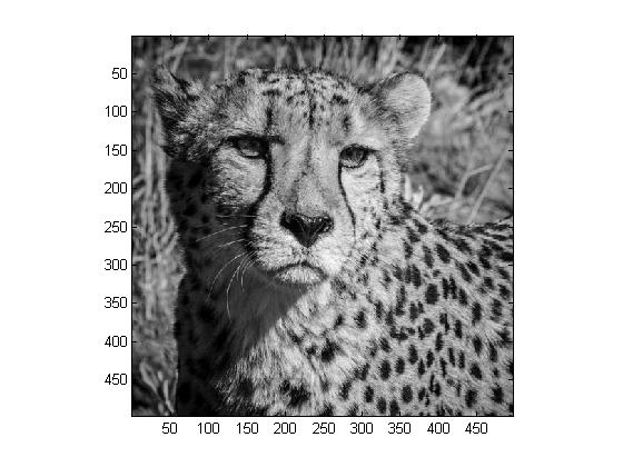
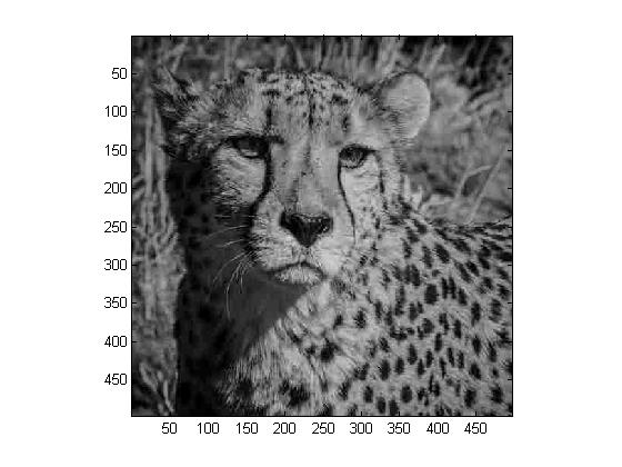
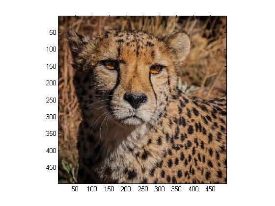
We will be using the above, \(496 \times 496\) photograph of a magnificent cheetah. Because our image has dimensions which are multiples of \(8\), cropping is not necessary. Therefore, we begin by converting our image to grayscale:
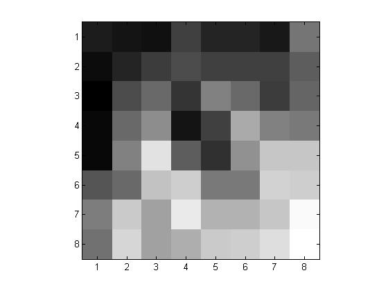
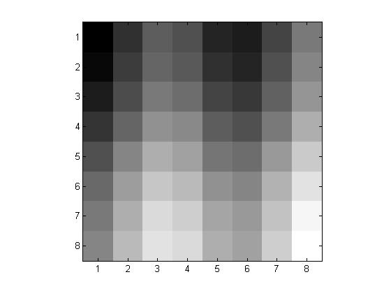
We then extract an \( 8 \times 8\) pixel block from our gray scale image using xb=x(81:88,81:88) along with imagesc:
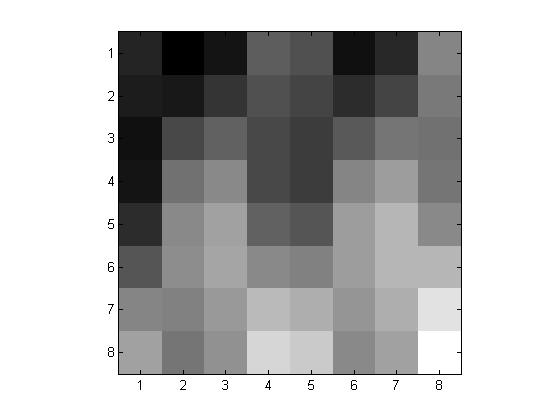
We will begin by working on our \( 8 \times 8\) pixel block. We want to apply the 2D-DCT asd well as quantization with \(p = 1, 2\) and \(4\) to obtain our \(Y_Q\) matricies. The following are the obtained images followed by their respective \(Y_Q\) matricies:

|
\(p=1\) \[ \left( \begin{matrix} -55 & -5 & 0 & -2 & -1 & 0 & 0 & 0\\ -12 & 1 & 0 & 0 & 0 & 0 & 0 & 0\\ 0 & 0 & 0 & 0 & 1 & 0 & 0 & 0\\ 0 & 0 & 0 & -1 & 0 & 1 & 0 & 0\\ 0 & 0 & 0 & 0 & 0 & 0 & 0 & 0\\ 0 & 0 & 0 & 0 & 0 & 0 & 0 & 0\\ 0 & 0 & 0 & 0 & 0 & 0 & 0 & 0\\ 0 & 0 & 0 & 0 & 0 & 0 & 0 & 0 \end{matrix} \right) \] |
|
\(p=2\) \[ \left( \begin{matrix} -27 & -3 & 0 & -1 & 0 & 0 & 0 & 0\\ -6 & 0 & 0 & 0 & 0 & 0 & 0 & 0\\ 0 & 0 & 0 & 0 & 1 & 0 & 0 & 0\\ 0 & 0 & 0 & 0 & 0 & 0 & 0 & 0\\ 0 & 0 & 0 & 0 & 0 & 0 & 0 & 0\\ 0 & 0 & 0 & 0 & 0 & 0 & 0 & 0\\ 0 & 0 & 0 & 0 & 0 & 0 & 0 & 0\\ 0 & 0 & 0 & 0 & 0 & 0 & 0 & 0 \end{matrix} \right) \] |
|
\(p=4\) \[ \left( \begin{matrix} -14 & -1 & 0 & -1 & 0 & 0 & 0 & 0\\ -3 & 0 & 0 & 0 & 0 & 0 & 0 & 0\\ 0 & 0 & 0 & 0 & 0 & 0 & 0 & 0\\ 0 & 0 & 0 & 0 & 0 & 0 & 0 & 0\\ 0 & 0 & 0 & 0 & 0 & 0 & 0 & 0\\ 0 & 0 & 0 & 0 & 0 & 0 & 0 & 0\\ 0 & 0 & 0 & 0 & 0 & 0 & 0 & 0\\ 0 & 0 & 0 & 0 & 0 & 0 & 0 & 0 \end{matrix} \right) \] |
We now want to carry out the steps above for all \( 8 \times 8\) blocks to reconstruct our entire gray scale image. The following are the obtained images:

|

|
|

|
For this entire step, we use MATLAB program Project5.m to work on our \(8 \times 8\) pixel block, and we use Project5a.m to tackle the entire image.
We are asked to modify our compression method from the previous step by using the JPEG compression matrix. The following are the obtained images:
|
|

|

|

|
For this entire step, we use MATLAB program Project5a.m.
For this step, we are asked to work on our original colored image. We carry out all of the steps from Step 1, only this time we have to account for colors Red, Green, and Blue separetely. The following are our results:

|

|

|

|
For this entire step, we use MATLAB program Project5b.m.
We are now asked to transform our RGB values from the previous step into luminance/color difference coordinates. We carry out the steps from Step 1, only this time we will be accounting for Y, U, and V separetely, as well as using JPEG quantization.
|
|

|
|

|
For this entire step, we use MATLAB program Project5c.m.