Solve the problems presented in Computer Problems on pages 513-514 of the text. Carry out 11.2, problems 3-6.
Overview
Compression of data allows for data to transfer quickly between two sources and is based on numerical methods. Specifically, compression requires the usage of a Discrete Cosine Transformation, often abbreviated DCT, which is a finite sequence of points represented by cosine functions with different frequencies. Also, quantization can be used to apply a filter, such a low pass frequency or high pass frequency, which will allow less bits to store data.In order to compression an image, such as in the JPEG format, quantization and discrete cosine transform is used. When implementing image compression in code, the image is indexed in terms of 8 x 8 blocks in which the data is compressed and then displayed. The sections below discuss the implementation and results of using DCT and JPEG compression.
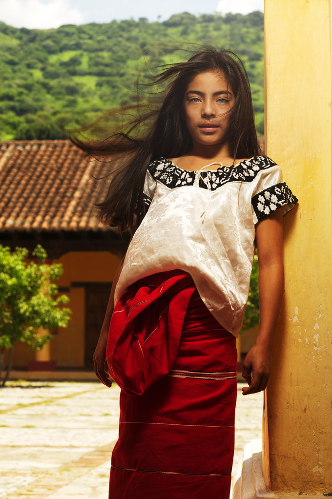
For this project, images were read into MatLab by using the built in imread function which saves the color values in red, green, and blue at each pixel location. The values of each color range from [0,255] by integers. This project utilizes transformations and quantizations on this color values which allows for digital compression. The main code can be downloaded and run in MatLab.
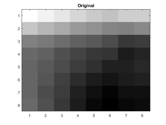
Part 1 - Grayscale 8x8 Image Compression by Quantization
For this portion of the Project, we are asked to explore the compression on an \(8\times 8\) section of our matrix, and then use that \(8 \times 8\) compression method to rebuild the entire image.
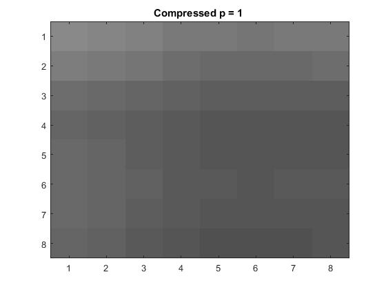
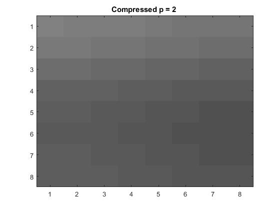
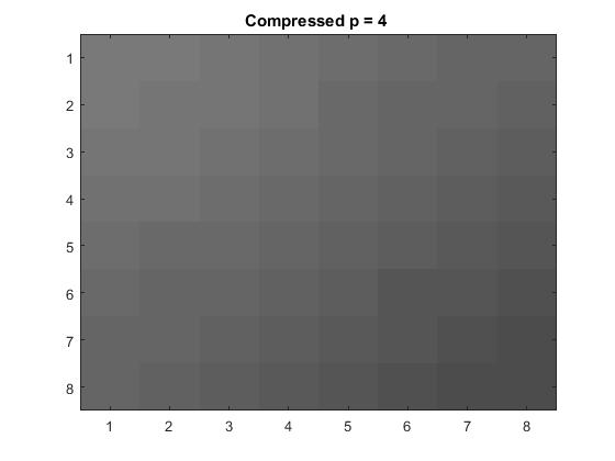
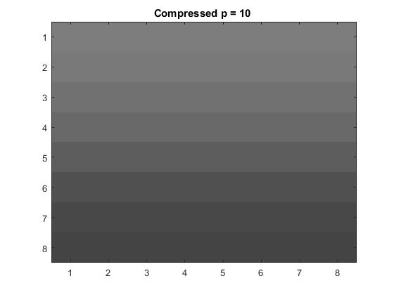
We extracted an \(8\times 8\) pixel block using MATLAB command \( xb=x(81:88,91:98) \), and ran trhough the linear quatization with loss parameter \(p=1,2,4\), and \(10\).
Quantization reduces the storage cost by assigning fewer bits to store information about the lower right corner of the transformation matrix, while still retaining the coefficients at a lower accuracy.
The quantization matrix Q calculates and assigns arbitrary number of bits allowed for each frequency.The loss parameter value is represented by \(p\). The larger this value the more information is lost to quantization. The method of 2D-DCT, (Discrete Cosine Transform) which reduces the number of bits representing each individual pixel on the image is applied to the original grayscaled 8x8 block in the quantization process. Then dequantization is used to reconstruct the block through inverse 2D-DCT.
For \(p=1,\ \) \(Y_Q=\begin{bmatrix} -29 & 3 & 1 & 0 & 0 & 0 & 0 & 0 \\ 5 & 0 & 0 & 0 & 0 & 0 & 0 & 0\\ 2 & 0 & 0 & 0 & 0 & 0 & 0 & 0 \\ 1 & 0 & 0 & 0 & 0 & 0 & 0 & 0 \\ 0 & 0 & 0 & 0 & 0 & 0 & 0 & 0 \\ 0 & 0 & 0 & 0 & 0 & 0 & 0 & 0 \\ 0 & 0 & 0 & 0 & 0 & 0 & 0 & 0 \\ 0 & 0 & 0 & 0 & 0 & 0 & 0 & 0 \\ \end{bmatrix}\)
For \(p=2,\ \) \(Y_Q=\begin{bmatrix} -15 & 1 & 0 & 0 & 0 & 0 & 0 & 0 \\ 3 & 0 & 0 & 0 & 0 & 0 & 0 & 0\\ 1 & 0 & 0 & 0 & 0 & 0 & 0 & 0 \\ 0 & 0 & 0 & 0 & 0 & 0 & 0 & 0 \\ 0 & 0 & 0 & 0 & 0 & 0 & 0 & 0 \\ 0 & 0 & 0 & 0 & 0 & 0 & 0 & 0 \\ 0 & 0 & 0 & 0 & 0 & 0 & 0 & 0 \\ 0 & 0 & 0 & 0 & 0 & 0 & 0 & 0 \\ \end{bmatrix}\)
For \(p=4,\ \) \(Y_Q=\begin{bmatrix} -7 & 1 & 0 & 0 & 0 & 0 & 0 & 0 \\ 1 & 0 & 0 & 0 & 0 & 0 & 0 & 0\\ 0 & 0 & 0 & 0 & 0 & 0 & 0 & 0 \\ 0 & 0 & 0 & 0 & 0 & 0 & 0 & 0 \\ 0 & 0 & 0 & 0 & 0 & 0 & 0 & 0 \\ 0 & 0 & 0 & 0 & 0 & 0 & 0 & 0 \\ 0 & 0 & 0 & 0 & 0 & 0 & 0 & 0 \\ 0 & 0 & 0 & 0 & 0 & 0 & 0 & 0 \\ \end{bmatrix}\)
For \(p=10,\ \) \(Y_Q=\begin{bmatrix} -2 & 0 & 0 & 0 & 0 & 0 & 0 & 0 \\ 1 & 0 & 0 & 0 & 0 & 0 & 0 & 0\\ 0 & 0 & 0 & 0 & 0 & 0 & 0 & 0 \\ 0 & 0 & 0 & 0 & 0 & 0 & 0 & 0 \\ 0 & 0 & 0 & 0 & 0 & 0 & 0 & 0 \\ 0 & 0 & 0 & 0 & 0 & 0 & 0 & 0 \\ 0 & 0 & 0 & 0 & 0 & 0 & 0 & 0 \\ 0 & 0 & 0 & 0 & 0 & 0 & 0 & 0 \\ \end{bmatrix}\)
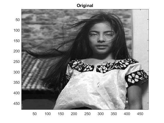
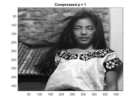
Part 2 - Grayscale Image Compression and Reconstruction
The same method we used for the \( 8 \times 8 \) block was implemented across the entire image for the reconstruction. The results of the linear quantization and compression is shown below:


Part 3 - Grayscale JPG Quantization
This section involves compression of a grayscale image using the JPEG recommended matrix as shown below:
For \(Q_{JPG} \ \) \(= p\begin{bmatrix} 16 & 11 & 10 & 16 & 24 & 40 & 51 & 61\\ 12 & 12 & 14 & 19 & 26 & 58 & 60 & 55 \\ 14 & 13 & 16 & 24 & 40 & 57 & 69 & 56 \\ 14 & 17 & 22 & 29 & 51 & 87 & 80 & 62 \\ 18 & 22 & 37 & 56 & 68 & 109 & 103 & 77 \\ 24 & 35 & 55 & 64 & 81 & 104 & 113 & 92 \\ 49 & 64 & 78 & 87 & 103 & 121 & 120 & 102 \\ 72 & 92 & 95 & 98 & 112 & 100 & 103 & 99 \\ \end{bmatrix}\)
The linear quantization matrix using the Hilbert matrix can be constructed using the MatLab command Q = p*8./hilb(8). While the JPEG linearization contains the matrix Q. Its values are determined based on the way human perceive visual images: Below are the compressed images through quantization using the linear quantization matrix and Annex K:


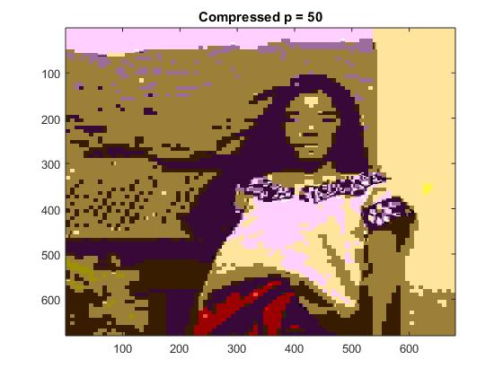
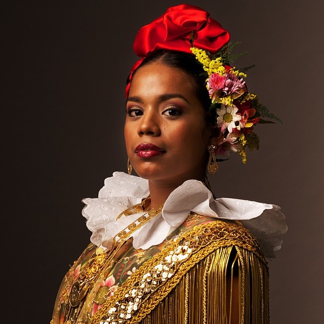
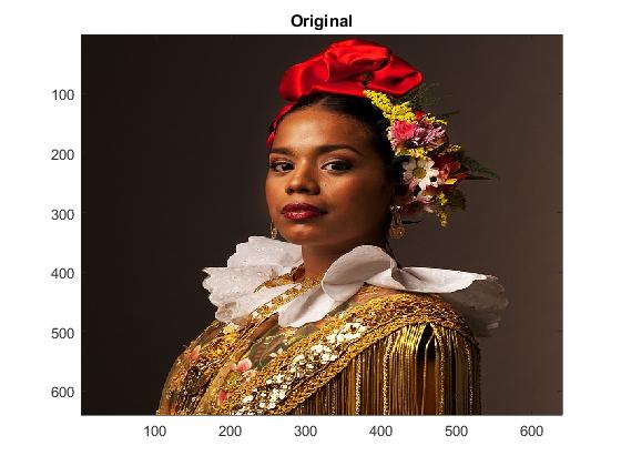
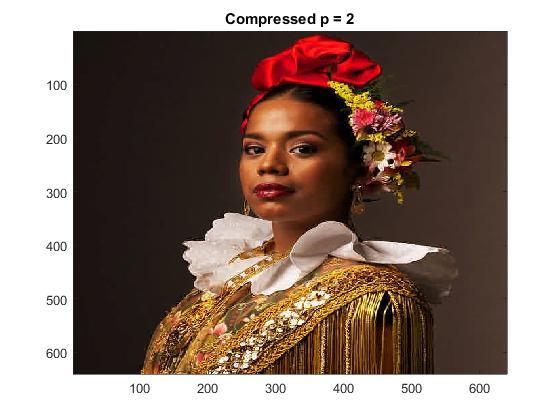
Part 4 - Color Image Compression
For color images, linear quantization, and dequantization are applied respectively to each R, G, B colors separately.


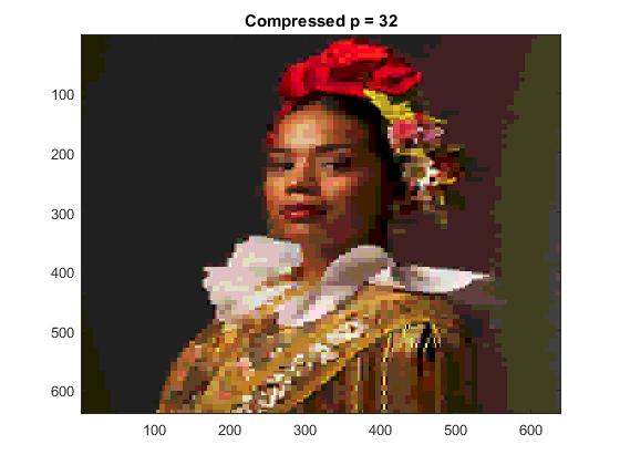
Part 5 - Luminance & Color Compression
Finally, in the last part we were asked to explore color image compression through the idea of luminance and the color differences. To do this, we used the JPEG suggested quantization matrix for Luminance Y:
For \(Q_y \) \(= p\begin{bmatrix} 16 & 11 & 10 & 16 & 24 & 40 & 51 & 61 \\ 12 & 12 & 14 & 19 & 26 & 58 & 60 & 55 \\ 14 & 13 & 16 & 24 & 40 & 57 & 69 & 56 \\ 14 & 17 & 22 & 29 & 51 & 87 & 80 & 62 \\ 18 & 22 & 37 & 56 & 68 & 109 & 103 & 77 \\ 24 & 35 & 55 & 64 & 81 & 104 & 113 & 92 \\ 49 & 64 & 78 & 87 & 103 & 121 & 120 & 102 \\ 72 & 92 & 95 & 98 & 112 & 100 & 103 & 99 \\ \end{bmatrix} \)
and the Color Difference Matrix for the color differences U and V:
For \(Q_{color} \ \) \(= p\begin{bmatrix} 17 & 18 & 24 & 47 & 99 & 99 & 99 & 99 \\ 18 & 21 & 26 & 66 & 99 & 99 & 99 & 99 \\ 24 & 26 & 56 & 99 & 99 & 99 & 99 & 99 \\ 47 & 66 & 99 & 99 & 99 & 99 & 99 & 99 \\ 99 & 99 & 99 & 99 & 99 & 99 & 99 & 99 \\ 99 & 99 & 99 & 99 & 99 & 99 & 99 & 99 \\ 99 & 99 & 99 & 99 & 99 & 99 & 99 & 99 \\ 99 & 99 & 99 & 99 & 99 & 99 & 99 & 99 \\ \end{bmatrix} \)
and Y, U and V are defined by:
\begin{eqnarray*} Y &=& 0.299R + 0.587G + 0.114B \\ U &=& B - Y \\ V &=& R - Y \\ \end{eqnarray*}
This YUV image is what is compressed, and then converted back to an RGB image using:
\begin{eqnarray*} R &=& V + Y \\ B &=& U + Y \\ G &=& \frac{(Y - 0.299R - 0.114B)}{0.587} \\ \end{eqnarray*}
The code can be found here.