Contents
clear; close all;
prefilt = [0.223755 0.552490 0.223755];
derivfilt = [-0.453014 0 0.45301];
blur = [1 1 1 1 1 1 1 1 1 1];
blur = blur / sum(blur);
nframes = 3;
[dimy,dimx]=size(readpgm('yos.10.pnm'));
seq(1).im = zeros(dimy,dimx);
for i=1:nframes
filename=sprintf('yos.%d.pnm',9+i);
seq(i).im=readpgm(filename);
end
Spatial and temporal derivative
f = zeros(dimy,dimx);
for i = 1 : nframes
f = f + prefilt(i)*seq(i).im;
end
fx = conv2( conv2( f, prefilt', 'same' ), derivfilt, 'same' );
fy = conv2( conv2( f, prefilt, 'same' ), derivfilt', 'same' );
ft = zeros(dimy,dimx);
for i = 1 : nframes
ft = ft + derivfilt(i)*seq(i).im;
end
ft = conv2( conv2( ft, prefilt', 'same' ), prefilt, 'same' );
blur = [1 6 15 20 15 6 1];
blur = blur / sum(blur);
fx2 = conv2( conv2( fx .* fx, blur', 'same' ), blur, 'same' );
fy2 = conv2( conv2( fy .* fy, blur', 'same' ), blur, 'same' );
fxy = conv2( conv2( fx .* fy, blur', 'same' ), blur, 'same' );
fxt = conv2( conv2( fx .* ft, blur', 'same' ), blur, 'same' );
fyt = conv2( conv2( fy .* ft, blur', 'same' ), blur, 'same' );
s = 4;
[ydim,xdim] = size( fx );
Ux = zeros( ydim/s, ceil(xdim/s) );
Uy = zeros( ydim/s, ceil(xdim/s) );
cx = 1;
x = zeros( ydim/s, ceil(xdim/s) );
y = zeros( ydim/s, ceil(xdim/s) );
for i=1:size(Ux, 1)
i_start = (i-1)*s + 1;
i_end = i*s;
for j=1:size(Ux, 2)
j_start = (j-1)*s + 1;
j_end = j*s;
G = [sum(sum(fx2(i_start:i_end, j_start:j_end))), ...
sum(sum(fxy(i_start:i_end, j_start:j_end))); ...
sum(sum(fxy(i_start:i_end, j_start:j_end))), ...
sum(sum(fy2(i_start:i_end, j_start:j_end)))];
b = [sum(sum(fxt(i_start:i_end, j_start:j_end))); ...
sum(sum(fyt(i_start:i_end, j_start:j_end)))];
u = G\(-b);
Ux(i,j) = u(1);
Uy(i,j) = u(2);
x(i,j) = j_end - s/2;
y(i,j) = i_end - s/2;
end
end
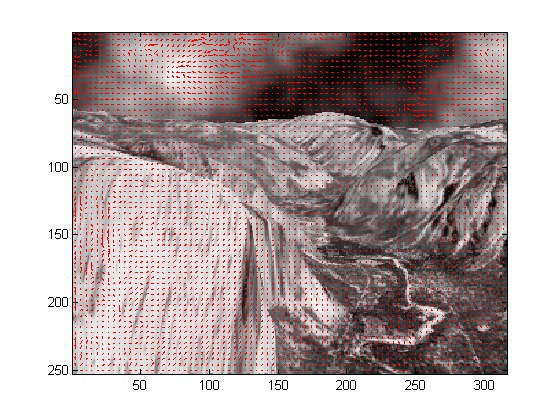
imagesc(seq(2).im);
colormap('gray');
hold on;
quiver(x, y, Ux, Uy, 'r');
set(gcf, 'color', 'w');