Project 3
COVID-19 Modeling and Maximum Likelihood Estimation
Description of project 3:
410Project3.pdf
Click to view the source code used for this proejct:
Question 1:
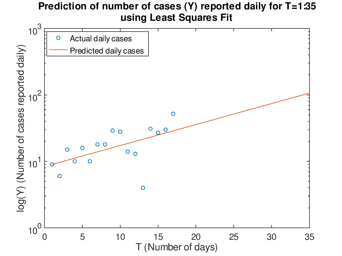
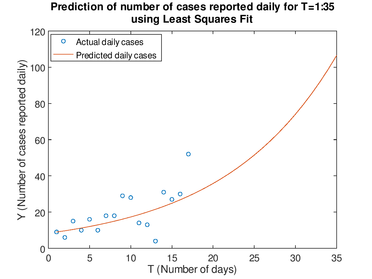
Find the best fit line using a least square fit.
Plot the data for T=1:17 and prediction for T=1:35 in both a normal and semilog plot using the least squares fit
The Least Square Fit model:
\[ \log Y = a_{1} + a_{2}T \approx 2.123762 + 0.072704T \]
Question 2:
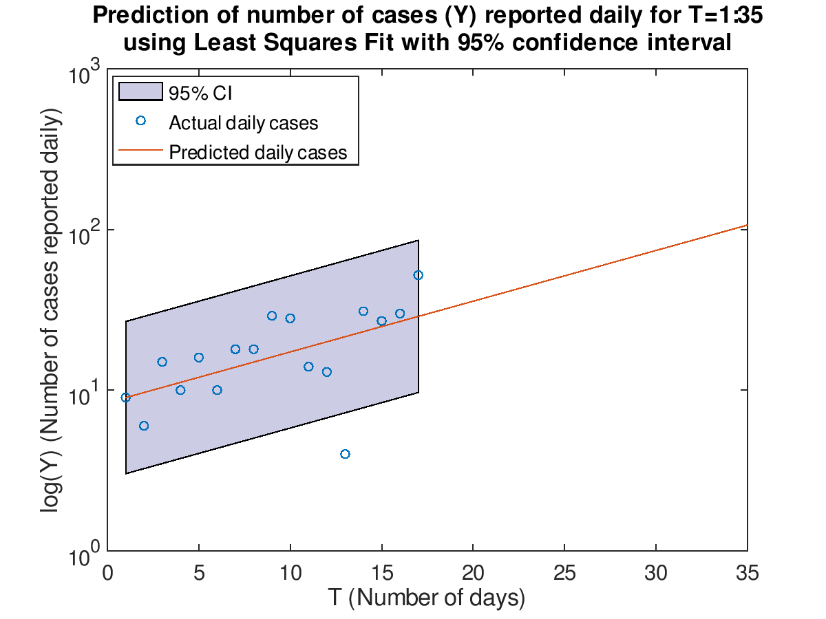
Compute the standard deviation to the Least Squares Fit and add the 95% confidence interval to the previous plots.
Question 3:
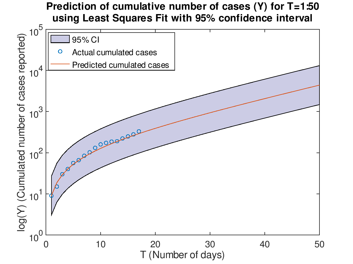
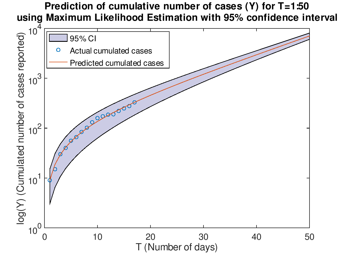
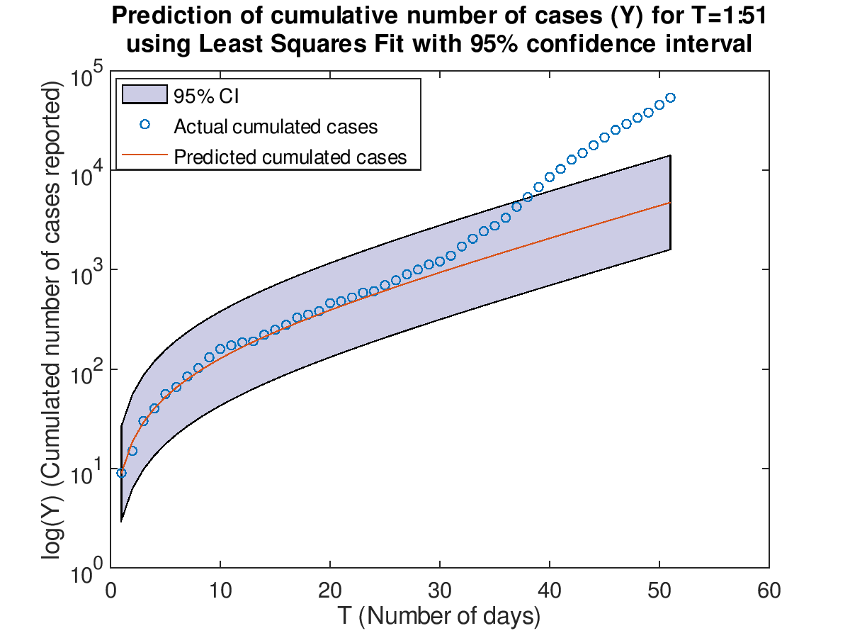
Plot the cumulative cases with prediction for T=1:50 with 95% confidence interval using Least Squares Fit.
Question 4:
In order to find the maximum likelihod estimates for \(a_1\) and \(a_2\),
we need to maximize \(L(a_1,a_2)\) by computing the gradient of \(L\) (\(\triangledown L\)).
The log-likelihood:
\[
L(a_1,a_2) = \log(P(Y_1, ..., Y_{17}|a_1,a_2)) = \sum^{17}_i=1 -e^{a_1 + a_2 T_i} + Y_i (a_1 + a_2 T_i) - \log(Y_i!)
\]
The Jacobian Matrix:
\[
\triangledown L =
\begin{bmatrix}
\frac{\partial L}{\partial a_{1}} \\
\frac{\partial L}{\partial a_{2}}
\end{bmatrix}
=
\begin{bmatrix}
\sum_{i=1}^{17} - e^{a_{1}+a_{2}T_{i}} + Y_{i} \\
\sum_{i=1}^{17} -T_{i} e^{a_{1}+a_{2}T_{i}} + Y_{i}T_{i}
\end{bmatrix}
\]
Question 5:
The Hessian Matrix:
\[
H(L) =
\begin{bmatrix}
\frac{\partial^{2} L}{\partial a_{1}\partial a_{1}} &
\frac{\partial^{2} L}{\partial a_{2}\partial a_{1}} \\
\frac{\partial^{2} L}{\partial a_{1}\partial a_{2}} &
\frac{\partial^{2} L}{\partial a_{2}\partial a_{2}}
\end{bmatrix}
=
\begin{bmatrix}
\sum_{i=1}^{17} - e^{a_{1}+a_{2}T_{i}} &
\sum_{i=1}^{17} -T_{i} e^{a_{1}+a_{2}T_{i}} \\
\sum_{i=1}^{17} -T_{i} e^{a_{1}+a_{2}T_{i}} &
\sum_{i=1}^{17} -T_{i}^2 e^{a_{1}+a_{2}T_{i}}
\end{bmatrix}
\]
Question 6:
Apply the multivariate Newton's method to solve for \(\triangledown L(\vec{a}) = \vec{0}\) using the data for T=1:17.
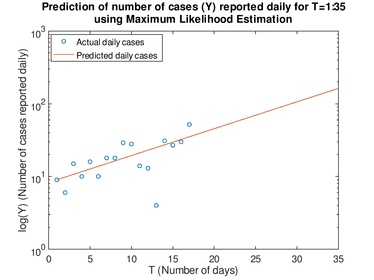
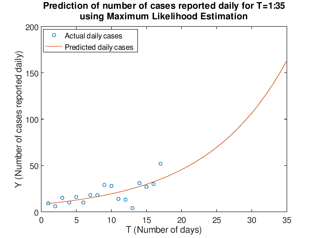
The maximum likelihood estimates for \(a_1 \approx 2.113807, a_2 \approx 0.085167\).
Question 7:
Plot the data for T=1:17 and prediction for T=1:35 in both a normal and semilog plot using the maximum likelihood estimation.
Question 8:
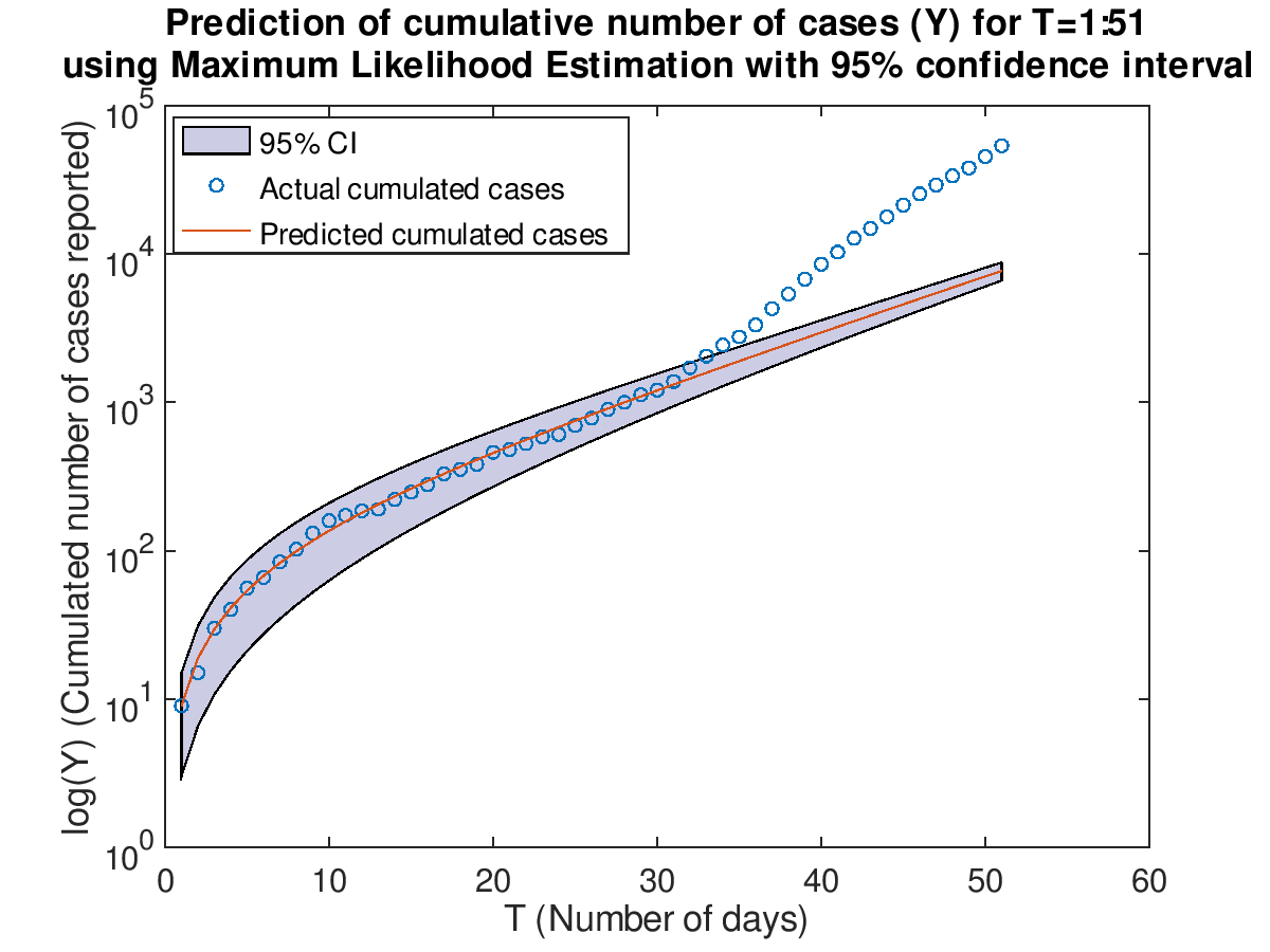
Retrieve the lastest data for the number of total COVID-19 cases outside of China.
Then use the two models which are trained on T=1:17 to make prediction on the cumulative cases. The latest
data retrieved is from February 7th to March 12th (T=1:51).
The maximum likelihood estimation has a smaller confidence interval than the least square fit. Both models
only perform better from T=1 to T=30. As T grows greater than 30, the number of cumulative cases increases
at the faster rate than the exponential rate. Overall, the maximum likelihood estimation model does better
than the least squares fit model because it has a smaller error range.
Question 9:
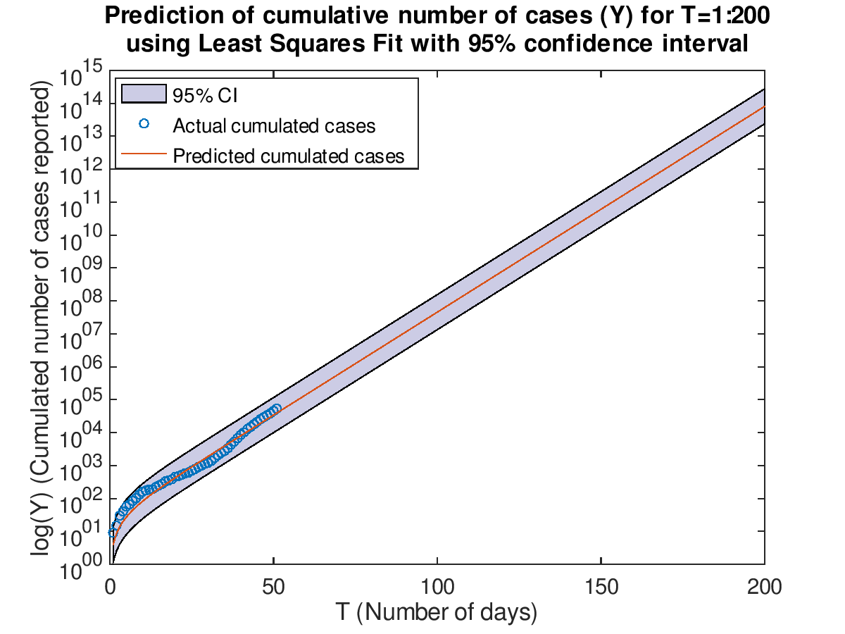
Refit both models using currently available data and run forecast out to 200 days.
Least Squares Fit: \( a_1 \approx 1.22733, a_2 \approx 0.14396 \)
Maximum Likelihood Estimation: \( a_1 \approx 0.59661, a_2 \approx 0.16495 \)
***Since the lower bound of the confidence interval contains some negative values
which are not valid in a logarithmic graph, the error bound is not filled here.
Conclusion:
The Least Squares Fit model predicts a million cumulative cases at about day 72.
The Maximum Likelihood Estimation predicts a million cumulative cases at about day 68.
Based on the previous check on updated data, both models predict successfully until day 30.
So for the updated models, they may predict successfully until day 80 depending on the rate of growth of the cases.