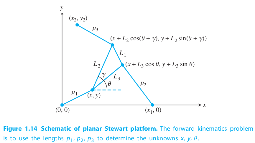
In this project, we simulated a simplified version of a Stewart platform. In our version, as opposed to six variable-length struts, we only account for three, which elevate and maneuver a triangular platform. The main goal of this project was to find the position of the platform, given the three strut lengths, by solving the forward kinematics problem. In this instance, this meant computing and for .
To start, we were given formulas for , derived using simple trigonometry: , , . In these formulas, , , , and .
Multiplying out the equations for and , substituting the first, then solving for and yields and , as long as .
Substituting these expressions for and into the equation for and multiplying by yields an expression . Finding the roots of we can easily determine the corresponding and values using the equations previously stated.
Part 1 of this project called for simply translating the formulas listed above into MATLAB code:
12345678910111213141516function [out,n1,n2,n3] = f1(theta,x,y2,L,gamma,p)
  A2 = L(3) * cos(theta) - x(1);
  B2 = L(3) * sin(theta);
  A3 = L(2) * cos(theta + gamma) - x(2);
  B3 = L(2) * sin(theta + gamma) - y2;

  N1 = B3 .* (p(2).^2 - p(1).^2 - A2.^2 - B2.^2) - B2.* (p(3).^2 - p(1).^2 - A3.^2 - B3.^2);
  N2 = -A3.* (p(2).^2 - p(1).^2 - A2.^2 - B2.^2) + A2.* (p(3).^2 - p(1).^2 - A3.^2 - B3.^2);
  D = 2 * (A2.*B3-B2.*A3);

  out=N1.^2+N2.^2-p(1).^2*D.^2;

  n1 = [N1/D,N2/D];
  n2 = [n1(1) + L(3)*cos(theta), n1(2) + L(3)* sin(theta)];
  n3 = [n1(1) + L(2)*cos(theta+gamma), n1(2) + L(2)* sin(theta + gamma)];
end
To test this code, we set the parameters , then substituted and ensured that :
12345678910111213141516171819L1 = 2;
L2 = sqrt(2);
L3 = L2;
L = [L1 L2 L3];

gamma = pi/2;

p1 = sqrt(5);
p2 = p1;
p3 = p1;
p= [p1 p2 p3];

x1 = 4;
y1 = 0;

x2 = 0;
y2 = 4;

x = [x1,x2];
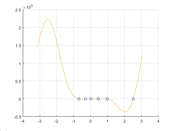
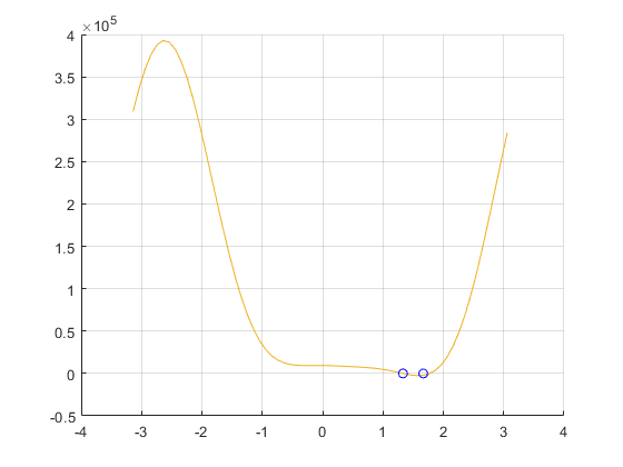
For Part 2, we plotted on the interval , ensuring that there were roots at as a check of our work:
123456789101112xint = -pi:0.1:pi;
out = @f1;
out1 = out(xint,x,y2,L,gamma,p);

figure(1)
plot(xint,out1)
hold on
grid
p2roots1 = secant_method(0,1,10,x,y2,L,p,gamma)
p2roots2 = secant_method(-1,0,10,x,y2,L,p,gamma)
plot([p2roots1 p2roots2],[0 0],'bo')
hold off
Running this code yielded the following:
12345678p2roots1 =

    0.7854


p2roots2 =

   -0.7808
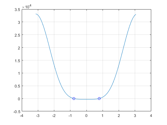
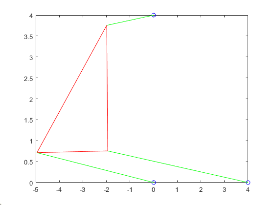
The roots returned by our code and displayed on the graph are equivalent to , so our results were sound.
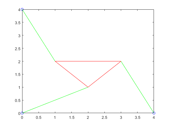
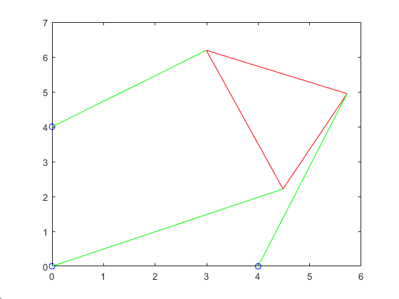
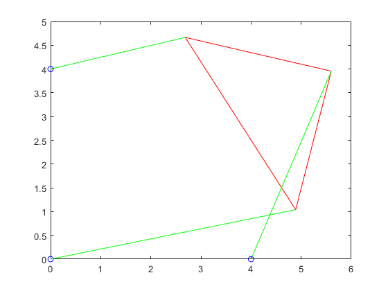
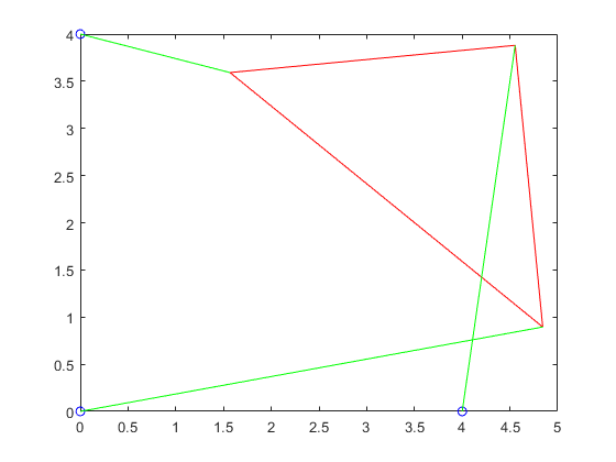
12p3struts1 = plotTriangle(p2roots1,x,y2,L,gamma,p,2)
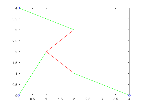
p3struts2 = plotTriangle(p2roots2,x,y2,L,gamma,p,3)
12345678910p3struts1 =

    2.2361    2.2361    2.2361
    2.2361    2.2361    2.2361


p3struts2 =

    2.2320    2.2320    2.2320
    2.2361    2.2361    2.2361
1234567891011121314151617181920212223242526272829303132function out=secant_method(theta0,theta1,i,x,y2,L,p,gamma)
y = @f1;
for(j=1:i)
theta2 = theta1 - ((y(theta1,x,y2,L,gamma,p) * (theta1 - theta0)) / ...
(y(theta1,x,y2,L,gamma,p) - y(theta0,x,y2,L,gamma,p)));
theta0 = theta1;
theta1 = theta2;
end out=theta1;
end
x = [5 0];
y2 = 6;
L = [3 (3*sqrt(2)) 3];
gamma = pi/4;
p = [5.0 5.0 3.0];
figure(4)
hold on
grid
out4 = out(xint,x,y2,L,gamma,p);
plot(xint,out4)
p5roots1 = secant_method(-.8,-.6,5,x,y2,L,p,gamma)
p5roots2 = secant_method(-.4,-.2,5,x,y2,L,p,gamma)
p5roots3 = secant_method(2,2.6,5,x,y2,L,p,gamma)
p5roots4 = secant_method(1,1.2,5,x,y2,L,p,gamma)
plot([p5roots1 p5roots2 p5roots3 p5roots4],[0 0 0 0],'bo')
hold off
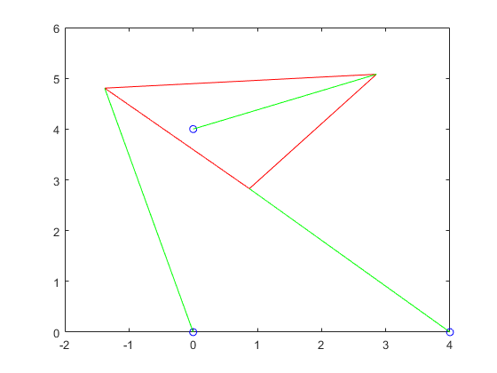
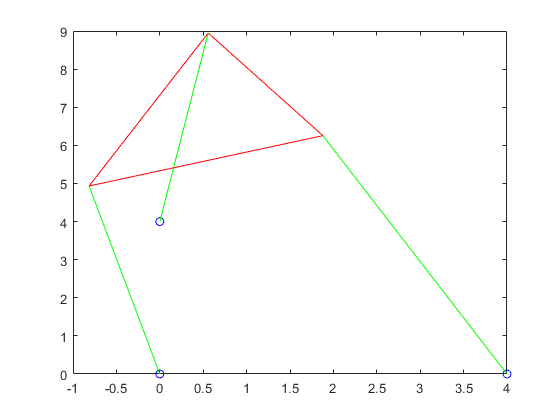
p5struts1 = plotTriangle(p5roots1,x,y2,L,gamma,p,5)
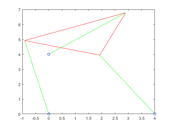
p5struts2 = plotTriangle(p5roots2,x,y2,L,gamma,p,6)
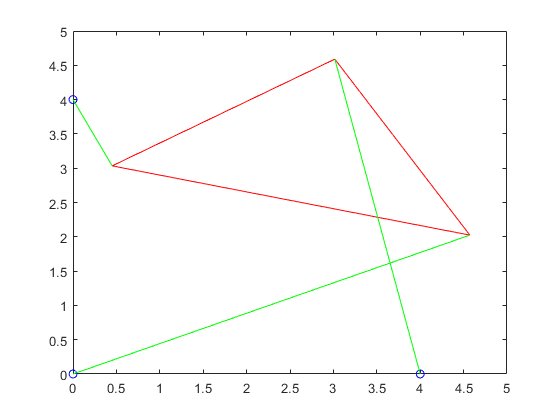
p5struts3 = plotTriangle(p5roots3,x,y2,L,gamma,p,7)
p5struts4 = plotTriangle(p5roots4,x,y2,L,gamma,p,8)
123456789101112131415161718192021222324252627282930313233343536373839404142p5roots1 =

   -0.7209


p5roots2 =

   -0.3310


p5roots3 =

    2.1159


p5roots4 =

    1.1437


p5struts1 =

    5.0000    5.0000    3.0000
    5.0000    5.0000    3.0000


p5struts2 =

    5.0000    5.0000    3.0000
    5.0000    5.0000    3.0000


p5struts3 =

    5.0000    5.0000    3.0000
    5.0000    5.0000    3.0000


p5struts4 =

    5.0000    5.0000    3.0000
    5.0000    5.0000    3.0000
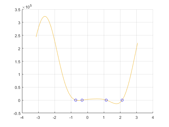
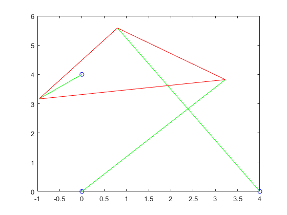
For this one, the functions are all the same as the previous ones, the only differences being that the structs that were hard coded in are changed, making 6 roots in stead of the 4 we saw in part 4.
123456789101112131415161718192021p(2) = 6.99;
figure(9)
hold on
grid
out5 = out(xint,x,y2,L,gamma,p);
plot(xint,out5)
p5roots1 = secant_method(-.8,-.6,5,x,y2,L,p,gamma)
p5roots2 = secant_method(-.4,-.2,5,x,y2,L,p,gamma)
p5roots3 = secant_method(-.2,.2,5,x,y2,L,p,gamma)
p5roots4 = secant_method(.3,.5,5,x,y2,L,p,gamma)
p5roots5 = secant_method(2,2.6,5,x,y2,L,p,gamma)
p5roots6 = secant_method(1,1.2,5,x,y2,L,p,gamma)
plot([p5roots1 p5roots2 p5roots3 p5roots4 p5roots5 p5roots6],[0 0 0 0 0 0],'bo')
hold off

p5struts1 = plotTriangle(p5roots1,x,y2,L,gamma,p,10)
p5struts2 = plotTriangle(p5roots2,x,y2,L,gamma,p,11)
p5struts3 = plotTriangle(p5roots3,x,y2,L,gamma,p,12)
p5struts4 = plotTriangle(p5roots4,x,y2,L,gamma,p,13)
p5struts5 = plotTriangle(p5roots5,x,y2,L,gamma,p,14)
p5struts6 = plotTriangle(p5roots6,x,y2,L,gamma,p,15)
12345678910111213141516171819202122232425262728293031323334353637383940414243444546474849505152535455565758596061626364p5roots1 =

   -0.6970


p5roots2 =

   -0.3035


p5roots3 =

    0.0139


p5roots4 =

    0.4560


p5roots5 =

    2.5128


p5roots6 =

    0.9780


p5struts1 =

    5.0000    6.9900    3.0001
    5.0000    6.9900    3.0000


p5struts2 =

    5.0000    6.9900    3.0000
    5.0000    6.9900    3.0000


p5struts3 =

    5.0000    6.9900    3.0000
    5.0000    6.9900    3.0000


p5struts4 =

    5.0000    6.9900    3.0000
    5.0000    6.9900    3.0000


p5struts5 =

    5.0000    6.9900    3.0000
    5.0000    6.9900    3.0000


p5struts6 =

    5.0000    6.9900    3.0000
    5.0000    6.9900    3.0000
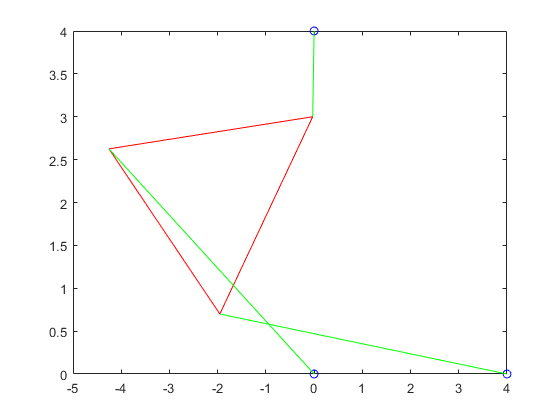
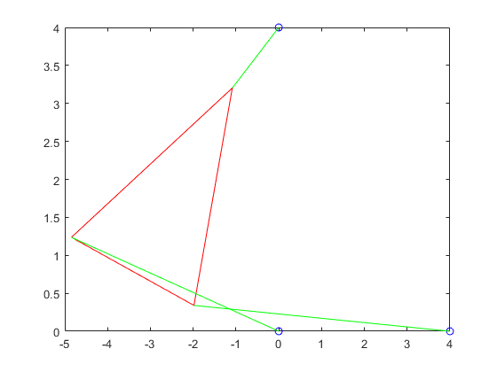
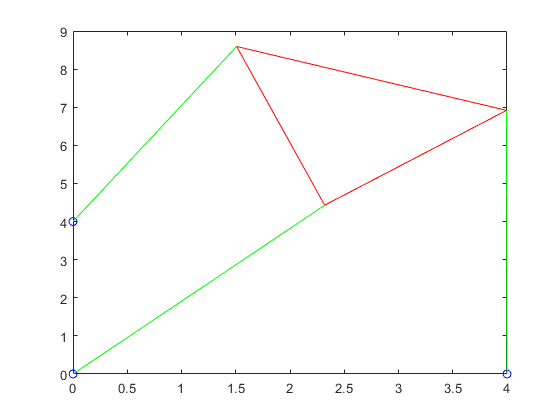
For this part, we had had to rewrite the function from part 1 to instead graph the possible s instead of the possible values for same goes all the other fuctions.
123456789101112p(2) = 4;
figure(16)
hold on
grid
out6 = out(xint,x,y2,L,gamma,p);
plot(xint,out6)
p6roots1 = secanat_method(1,1,5,5,x,y2,L,p,gamma)
p6roots2 = secanat_method(1,5,2,5,x,y2,L,p,gamma)
plot([p6roots1 p6roots2], [0 0], 'bo')
hold off
p6struts1 = plotTriangle(p6roots1,x,y2,L,gamma,p,17)
p6struts2 = plotTriangle(p6roots2,x,y2,L,gamma,p,18)
Sauer, T. (2018). Numerical Analysis (3rd ed.) Boston: Pearson.