Monte Carlo simulation and stochastic differential equation models are used extensively in financial calculations. In project 5, we will be employing both in the context of the Black-Scholes equation in order to calculate the value of call options.
As a reference, an option, be it a call or a put, is respectively the right to buy or sell a share of stock at a predetermined price, conventionally referred to as the strike price, at a future point in time, known as the exercise date. These particular financial instruments are commonly purchased and sold by both corporations and individual investors as a method of hedging risk, since they effectively enable investors to easily and dually invest in mutually exclusive financial market outcomes.
In the context of a call option, a $20 call for Generic Inc. stock in June, is the right to buy one share of stock in June at the rate of $20. If we suppose the current price of Generic Inc. stock is $18 per share, then questions concerning the value of the call option follow naturally. On the exercise date in June, the value of a $K call is clearly the max(\(X\)-\(K\),0), where \(X\) is the current market price of the stock. However, difficulty arises when considering the value of such a call prior to the exercise date, which is the case in our example.
In the 1960s, Fisher Black and Myron Scholes resourcefully applied the intuition behind Brownian motion to the topic of Asset Prices, and were awarded the Nobel Prize in Economics in 1997 for their discovery, which is eponymously dubbed the Black-Scholes model. One consequence of the Black-Scholes model is the so-called Black-Scholes formula, which is ubiquitously used in the practice of finance to accurately value stock options.
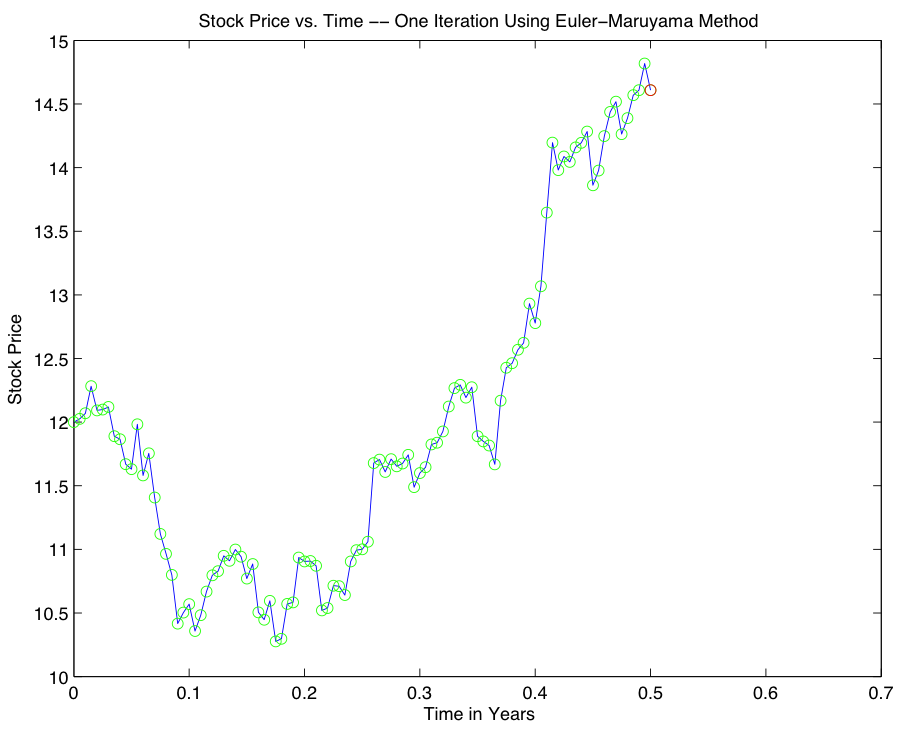
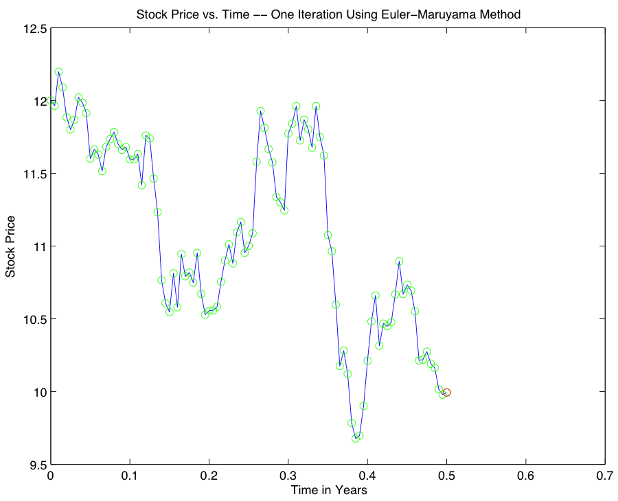
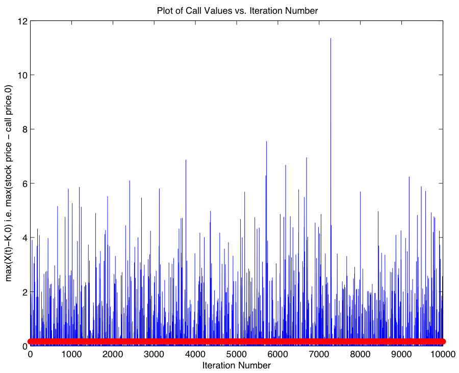
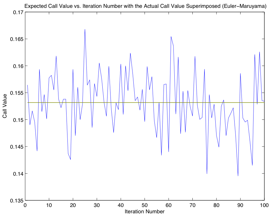
We are tasked with performing a Monte Carlo simulation in order to compute the expected value $$C(X,T) = e^{-rT} E(max(X(T)-K, 0)),$$ where \(r\) is the prevailing interest rate, \(T\) is the expiration date, \(X\)(\(T\)) is the stock price, and \(K\) is the call value. One required step in computing the expected value involves approximating the solution of the Stochastic Differential Equation $$dX = rX dt + \sigma X dB_t,$$ where \(\sigma\) corresponds to the diffusion constant, or volatility. We accomplish this task using the Euler-Maruyama method for SDEs, $$w_{i+1} = w_i +rw_i(\Delta t_i) + \sigma w_i(\Delta B_i),$$ and carry out 10000 iterations of the Monte Carlo simulation in deriving our approximation to the expected value problem. In order to demonstrate the moving parts included in the calculation, here are a few successive iterations of the Euler-Maruyama Method, demonstrating the stochastic nature of the differential equations of interest.
With the aim of computing the expected value in mind, we use the stock price at the expiration date for each of the 10000 iterations to compute the \(max(X(T) - K, 0)\) in each instance, and use the associated mean in our calculation. Proceeding in this fashion, we obtain an expected value of 0.157516386920192 in one instance; however, do note that the stochastic nature of the problem results in heterogeneous solutions. Code for Part 1
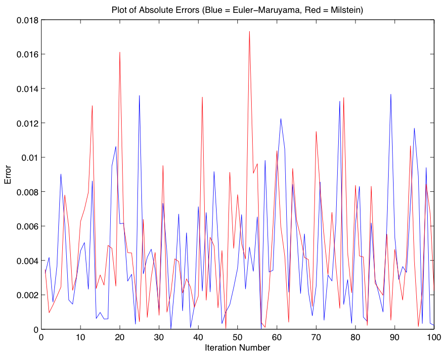
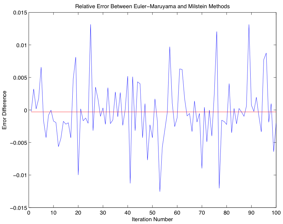
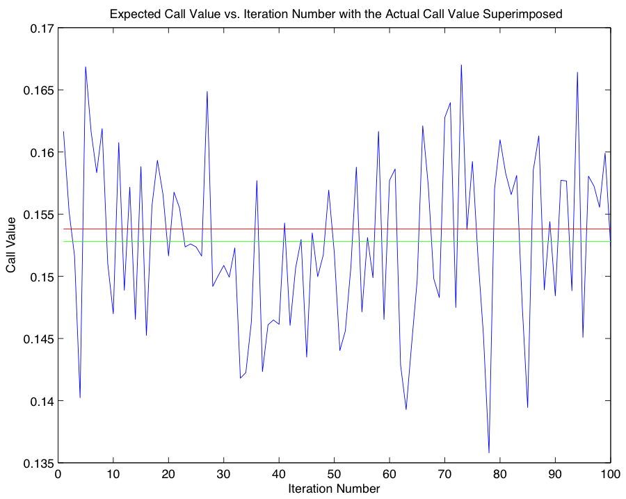
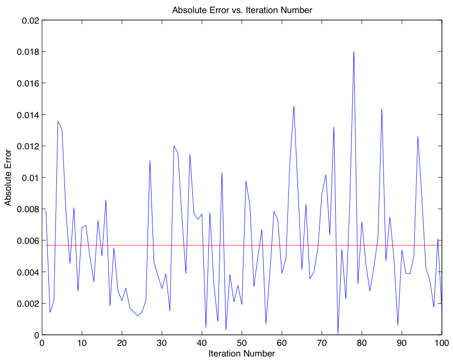
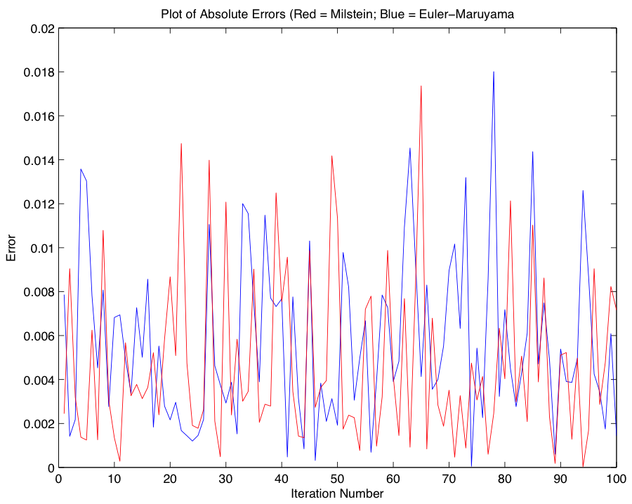
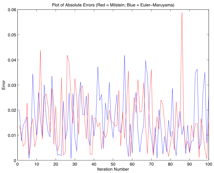
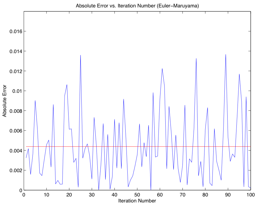
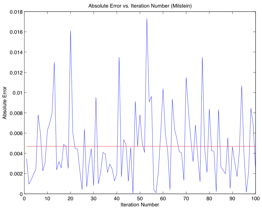
Since the solution we derived depends on calculating the expected value for \(X(T)\), we now turn our attention to the task of comparing our approximation with the closed-form expression for the call price, known as the Black-Scholes formula: $$C(X,T) = XN(d_1) - Ke^{-rT} N(d_2),$$ where \(N(X)\), \(d_1\), and \(d_2\) are defined as follows: $$N(X) = \frac{1}{2\pi} \int_{-\infty}^x e^{-s^2/2}ds,$$ $$d_1 = \frac{ln(X/K) + (r + \frac{1}{2}\sigma^2)T}{\sigma \sqrt{T}},$$ $$d_2 = \frac{ln(X/K) + (r - \frac{1}{2}\sigma^2)T}{\sigma \sqrt{T}}.$$ To gain an accurate picture of the error associated with the Euler-Maruyama Method, we complete 100 iterations of the approximation in part 1 for use in our comparison with the closed-form solution 0.153806238735601. The ensuing graphs represent the error between the closed-form solution and each iteration of our approximation. Code for Part 2
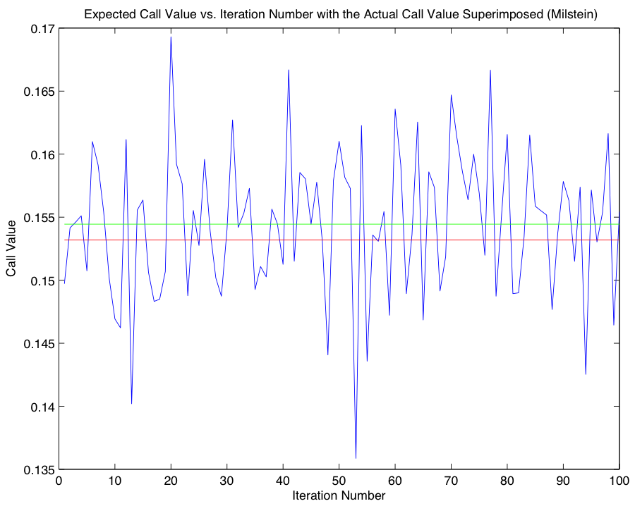
With an idea of the magnitude of error associated with our approximation using the Euler-Maruyama method, we now compare our results using the Euler-Maruyama Method with results obtained using a different SDE solver, the Milstein Method: $$w_{i+1} = w_i +rw_i(\Delta t) + \sigma w_i(\Delta B_i) + \frac{1}{2}\sigma^2w_i((\Delta B_i)^2 - \Delta t).$$ In order to provide an idea of the behavior of our new method, we first provide Milstein analogues to the graphs from Part 2, and leave our treatment of the comparison until afterwards.

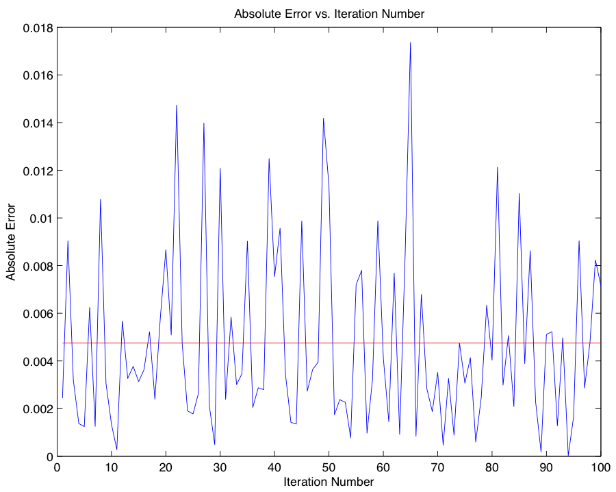
In comparing the accuracy of the alternative methods, we find that Milstein is more accurate in the few trials we performed, however without a significant number of additional trials it would be myopic to make conclusive probabilistic assertions; in fact, since the Euler-Maruyama and Milstein Methods are SDE solvers, their outputs are non-deterministic, and thus in any finite comparison of their accuracy it is possible for either method to outperform the other. Code for Part 3

A put option, in contrast to a call option, is the right to sell a share of stock at the strike price; its value is defined in the following manner: $$P(X,T) = e^{-rT} E(max(K - X(T), 0)),$$ where each variable is defined as in Part 1, and where X(T) is once again obtained by performing a Monte Carlo simulation. As in the case of a call option, we once again compute the expected value using both the Euler-Maruyama and Milstein Methods, and compare our approximations to the closed-form expression for the put price, $$P(X,T) = Ke^{-rT} N(-d_2) - XN(-d_1),$$ where each variable is defined as in Part 2. Proceeding in an identical fashion, we obtain the following approximations for the put value using the Euler-Maruyama and Milstein Methods respectively, and compare them with the closed-form solution 2.7835:
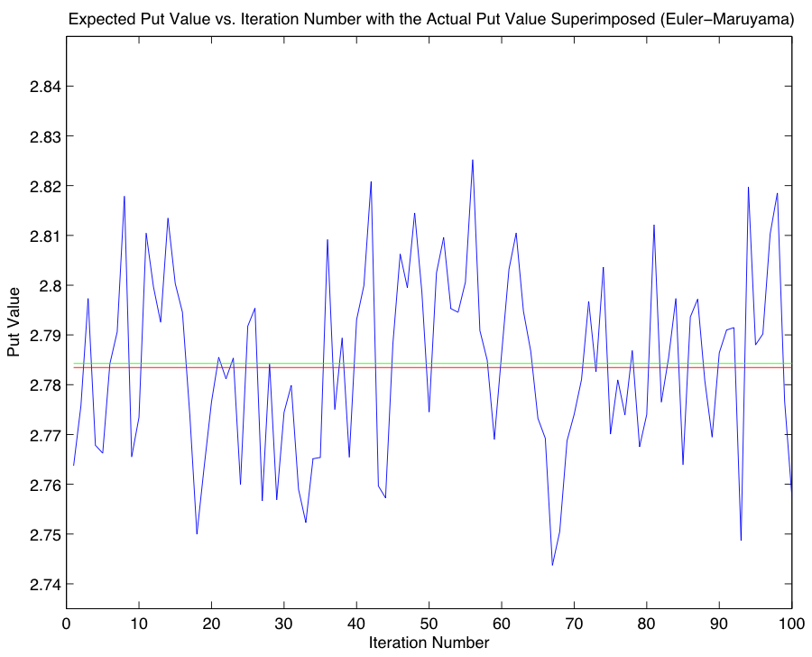
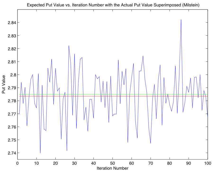
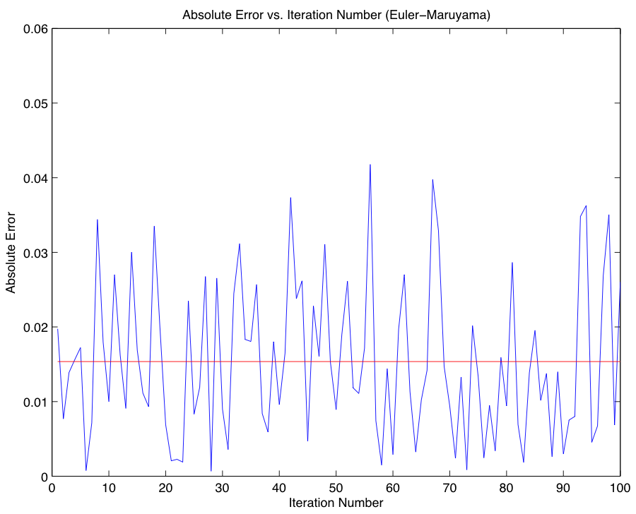

As argued in Part 3, the relative performance of the two methods is non-deterministic, and thus contrary to our previous findings regarding the accuracy of the respective SDE solvers, we find in the case of our put value approximations that the Euler-Maruyama Method is more accurate. Code for Parts 4 & 5

In addition to the standard call option discussed in Parts 1-3, there exist other variations in practice. One such variation is the down-and-out barrier option, which differs from the conventional call option in one fundamental way; in the case of the barrier option, the payout is canceled if the stock price falls below a threshold level, or price floor. For our purposes, this amounts to throwing out, or setting to zero, all iterations of the Euler-Maruyama and Milstein Methods that fall below a specified price at any time interval, regardless of their value at expiration time. As one would expect, this effectively reduces the expected value of the call option since we are discarding a comparatively small proportion of realizations of the call value which are otherwise positive. Once again, we treat the valuation problem with both the Euler-Maruyama and Milstein Methods, and compare our approximations with the closed-form solution given by: $$V(X,T) = C(X,T) - (X/L)^{1-2r/\sigma^2} C(L^2/X,T),$$ where \(L\) is the barrier value, and all other inputs are defined as above. Using the Euler-Maruyama and Milstein Methods we once again compute the following approximate solutions, and compare them with the closed-form solution 0.1532.
As in the previous problem, we find the Euler-Maruyama Method to be more accurate in this instance. Code for Part 6