Image Compression can be achieved by the use of the two dimensional
Discrete Cosine Transform(DCT), which is just the one dimensional DCT in
two dimensions. The DCT is often used to compress small blocks of an
image, as small as 8 by 8 blocks. So the image being used must have
dimensions that are divisible by 8. Some of the information from the block
is ignored, that is, the compression is lossy. The advantage of using the
DCT is that it helps organize the information so that the part that is
ignored is the part the human eye is least sensitive to. In other words,
the DCT will show us how to interpolate the data with a set of basis
functions that are in descending order of importance as far as the human
visual system is concerned.
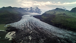
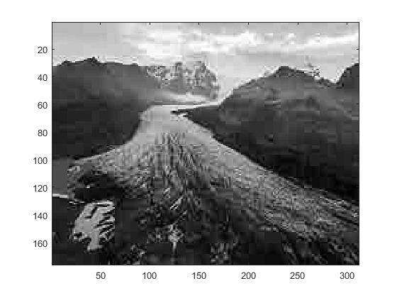
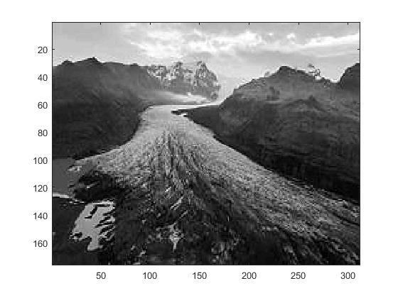
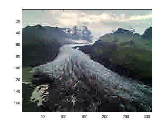
The following image of the breathtaking aerial view of Iceland's largest
glacier was selected for this project:
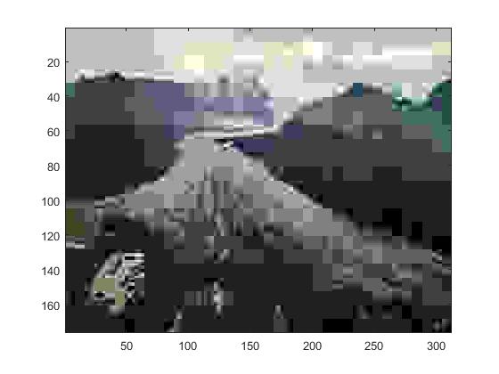
The above 640 by 360 image was resized, but maintianing the ratio aspect
so that we still have dimensions divisible by 8, so that when the image is
coverted to double reals precision, as we will see from Step 1, the image
dimensions do not exceed to 1000 pixels and an 8 by 8 block of the image
can be reconstructed through quatization and dequatization, as seen in Steps 1, 2 and
3 part D. The following 312 by 176 image was used throughout this project:
Computer Problems 11.2: 3-6
Step 1: Problem 3-Compressing a gray scale image with dimensions that
are divisible by 8
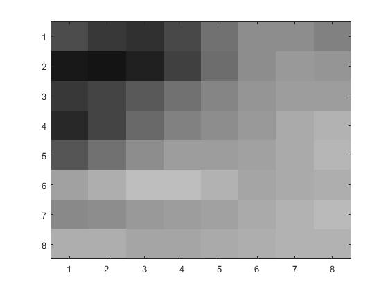
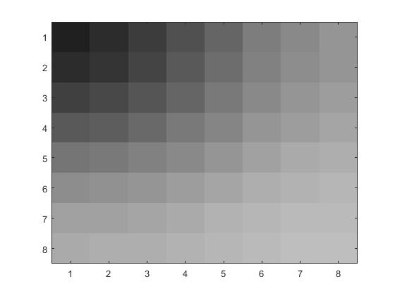
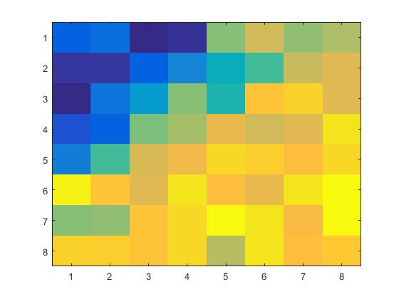
Part A: Displaying the extracted 8 by 8 block
The MATLAB code used for this part and parts c)-d) can be found
here.
The MATLAB Command X=xgray(81:88), in the case of this step was used to
extract an 8 by 8 block from the selected image above. The following image
of the block was what resulted:
Part C: Quantization by using linear quantization for three values of
p:
Linear quantization matrix:
$$
Q_c = p
\begin{bmatrix}
8 & 16 & 24 & 32 & 40 & 48 & 56 & 64 \\
16 & 24 & 32 & 40 & 48 & 56 & 64 & 72 \\
24 & 32 & 40 & 48 & 56 & 64 & 72 & 80 \\
32 & 40 & 48 & 56 & 64 & 72 & 80 & 88 \\
40 & 48 & 56 & 64 & 72 & 80 & 88 & 96 \\
48 & 56 & 64 & 72 & 80 & 88 & 96 & 104 \\
56 & 64 & 72 & 80 & 88 & 96 & 104 & 112 \\
64 & 72 & 80 & 88 & 96 & 104 & 112 & 120 \\
\end{bmatrix}
$$
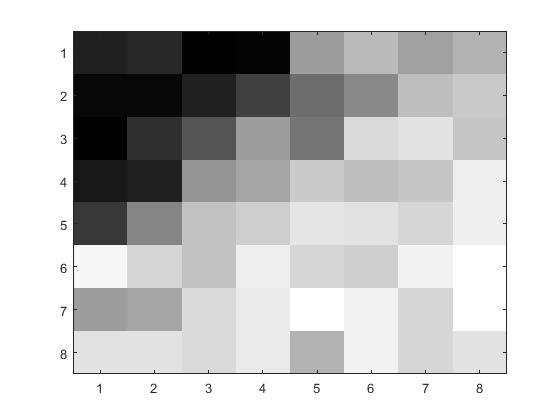
The value p represents the loss parameter and it is expected that the
higher the value we choose for p, the more destructed and blurry our
resulting compressed image will appear.
In MATLAB, the above matrix is defined by Q=p*8./hilb(8).
The following matrixes \(Y_Q\) were found for the three specified values
of p below:
The MATLAB Code that was used to produce the compressed images below can
be found here.
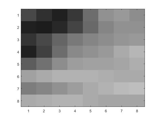
For p = 1:
For p = 2:
For p = 4:
As expected, the quality of the original grayscale image slowly begins to
deteriorate with higher values of p, that is, the image begins to become
deconstructed.
Step 2: Problem 4- Grayscal Compression using the JPEG
Quantization Matrix
The same MATLAB code that was used in Step 1 Part A, c and D was used to
produce the following image below and also to find the matrices in part C
and to find the reconstructed blocks in part D, with the difference that
the JPEG-suggested matrix above was used in place of the linear
quantization matrix.
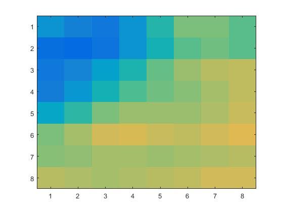
Part D: Reconstructed blocks of the color image for the specified
value of p
p = 1
p = 2
p = 4
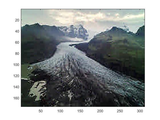
Part E: Reconstructing the entire image:
The MATLAB Code that was used for the color compression of the images can
be found here.
For p = 1
For p = 2
For p = 4
As what had happened in Step 1: Problem 3 Part E with our grayscale image,
our color image here also begins to become deconstructed with increasing
values of p.
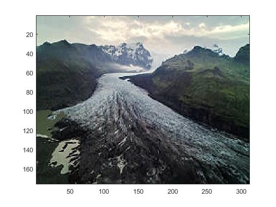
Step 4: Computer Problem 6- Color Image Compression for Y, U and V
Luminance
Coordinates
The MATLAB Code used for the YUV compression of the original image can be
found here
For p =1
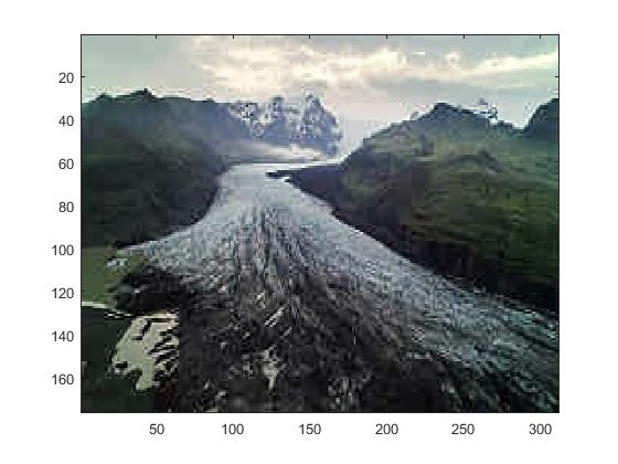
For p = 2
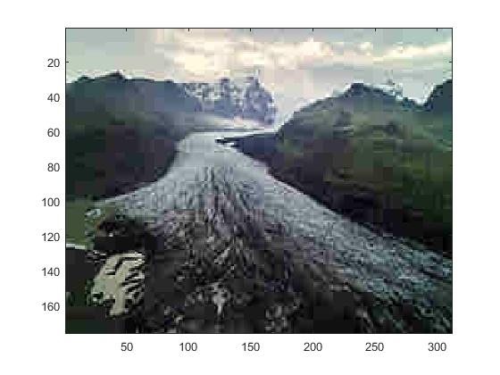
For p = 4
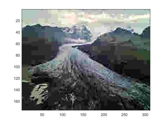
For p = 8
For p = 16
For p = 32
The sequence of the above images with their corresponding values of p show
that after a certain large value of p, the image begins to become
pixelated and almost destructed.


 As expected, the quality of the original grayscale image slowly begins to
deteriorate with higher values of p, that is, the image begins to become
deconstructed.
As expected, the quality of the original grayscale image slowly begins to
deteriorate with higher values of p, that is, the image begins to become
deconstructed.

 As what had happened in Step 1: Problem 3 Part E with our grayscale image,
our color image here also begins to become deconstructed with increasing
values of p.
As what had happened in Step 1: Problem 3 Part E with our grayscale image,
our color image here also begins to become deconstructed with increasing
values of p.