Introduction: This project examines the GPS and the errors associated with the transmitted times from the satellites. We wrote MATLAB code to calculate the maximum time and postition errors produced in transmission for the satellites.
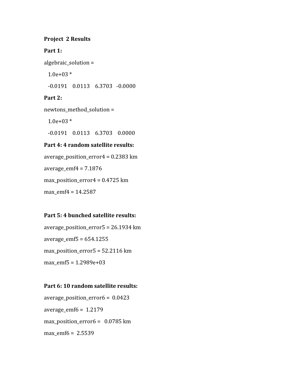
1. The goal of part one was to calculate the position of a GPS device algebraically. Given the positions of 4 satellites, and the equation relating satellite to GPS positions, it is possible to construct a solvable linear system of equations. The solution to this equation is a 3x2 matrix, which defines x, y, and z in terms of the variable d. This result can be used to simplify one of the satellite equations, such that the only variable is d, and this degree 2 expression can be solved using the quadratic formula. All of the results were generated from the main.m SolveGPS.m: Generates a linear system of equations and selects the correct root found by the quadratic forumula. SolveGPSQuadratic.m: Solves the degree 2 satellite equation, simplified in terms of d.
3. In part three, we calculated the position of the GPS device using the Multivariate Newton's Method. Given a set of satellite equations, it is possible to calculate the Jacobian matrix J, and the residual matrix R. Then, the next estimate of the position can be computed using x_next = x_current - J\R. Again, we use main.m to genreate the results. NewtonsMethodGPS.m: Calculates an improved position estimate over multiple iterations. SatellitesJacobianMatrix.m: Computes the Jacobian matrix for a set of satellite equations at a given position. EvaluateSatelliteEquations.m: Computes the residual matrix for the satellite equations at a given position.
4. In part 4, we change to spherical coordinates and redefine the initial satellite positions. This utilized a new part of code to parts 1 and 3, SphericalConversion.m . Our values for phi and theta were determined randomly, with phi between 0 and pi/2 and theta between 0 and 2*pi. We found the ranges of the satellites, along with the travel times. From this, we calculated the error magnification factor ( EMF.m ), the position error of the GPS location, and the condition number. Our results for delta t_i = 10^{-8} gave a condition number of 14.2587 and a maximum postion error of 472.5 m.
5. This part involved the same calculations as in part 4, but the satellites were bunched closely together. To obtain the different positions, we chose an initial value for theta (1) and phi (2*pi), then chose the other values within 5% of the initial value. Here, the results gave a condition number of 1.2989e3 and a maximum position error of 52,211.6 m. There was a significant increase in both values, which indicates that to to reduce the postion error given by the GPS, the satellites should be loosely bunched together.
6. We found that when the number of satellites increased to 10, the condition number decreased dramatically to 2.5539 and the position error was 78.5 m with an initial vector of [50, 50, 6300, 0.0003]. This result was significantly less than the four loosely and tightly bunched satellites from parts 4 and 5, leading to the conclusion that increasing the number of loosely bunched satellites is the best way to maintain accuracy while using GPS. We would guess that the maximum postion error given by the GPS, using more satellites, would be around 80 m, based on our results.
Conclusion: We were able to calculate satellites positions algebraically and numerically, and also find the error in position and condition number associated with each. Additional Code: BackSolve.m SolveAxEqualsb.m GaussianElimination.m Division of Labor: Stephen wrote the computer codes for parts 1, 3 and 6. Avis wrote SphericalToCartesian.m and did the calculations for condition number and max position error in parts 4 and 5. Both Stephen and Avis analyzed the results.