For this project, we chose to focus on the Kinematics of the stewart platform. Essnetially, the kinematics problem applied to a stewart platform revolves around solving for x,y and θ, given the lengths of the three struts, p1, p2, and p3. The project specs provided numerous equations, but the most important equations were in terms of θ, which later allowed us to solve for x and y. Primarily, the following sample equations below were useful for solving the problem once we attained the appropriate thetas:
Based on the MATLAB function that our group created for f(θ), we yielded a return value of -4.5475 e-13 for both arguments of π/4 and -π/4. In our implementation of the function, theta was the sole parameter, whereas L1, L2, L3, Gamma, x1, x2, and y2 were all treated as fixed constants local to the function. Since the return value of the function was -4.5475e-13, which is essentially 0, we can conclude that our group's implementation of the function was indeed correct. This function is later used with the bisection method to determine the roots, which are the appropriate poses for finding constructing 4 proper planar Stewart platforms with the given
After concluding that the function was implemented correctly, we plotted f(θ) on the interval from [-π, π]. We were also able to verify based on the plot of the function that f(-π/4) and f(π/4) are indeed 0. The plot can be seen below:
After reproducing Figure 1.15 (Page 69) via MATLAB, the following plots were produced:
For problem four, we updated the fixed constant variables within our original function to be equal to the following values: <\br>
x1 = 5, (x2, y2) = (0,6),L1 = L3 = 3,L2 = 3√2,γ = π/4,p1 = p2 = 5,p3 = 3<\br>
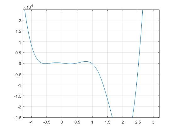
Upon updating our function, we were able to first plot the function for all possible thetas on the range of [-π, π] to produce the plot below. This plot below indicates that the function has 4 roots, where the roots are corresponding with the appropriate poses in context of the problem.
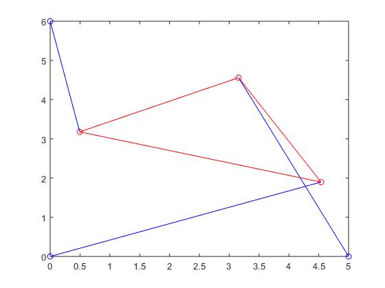
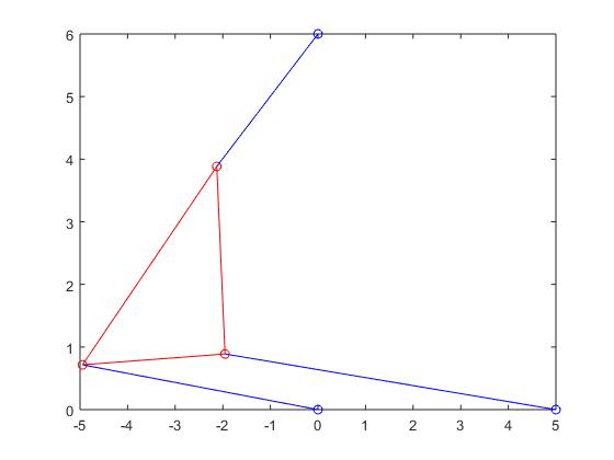
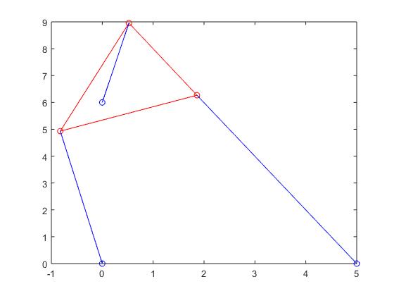
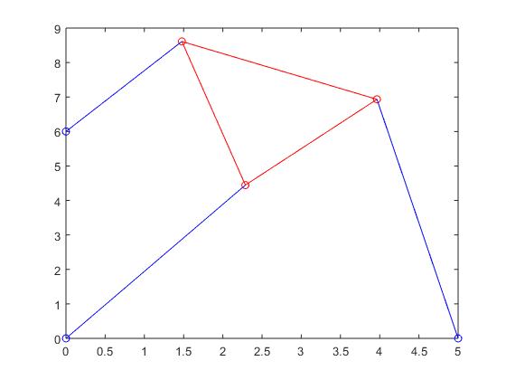
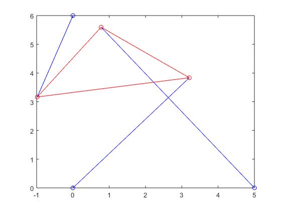
 Via the bisection method, we were able to use guessing and checking based on the graph produced above to determine the roots. Essentially, the bisection method, with the method signature of bisect(f,a,b,tol) was calling the function we initiallly created, along with possible intervals a and b (which we guessed based on the plot), and also the tolerance. By using the plot above and the bisection method, we were able to generate four distinct roots or poses: -0.9376, -0.0592, 1.1569, 2.0495 . Once we obtained these poses (aka roots), we were able to use the values to determine the values of x and y (as seen in figure 1.14). The new Stewart Platforms generated with the appropriate poses can be seen below, in respective order:
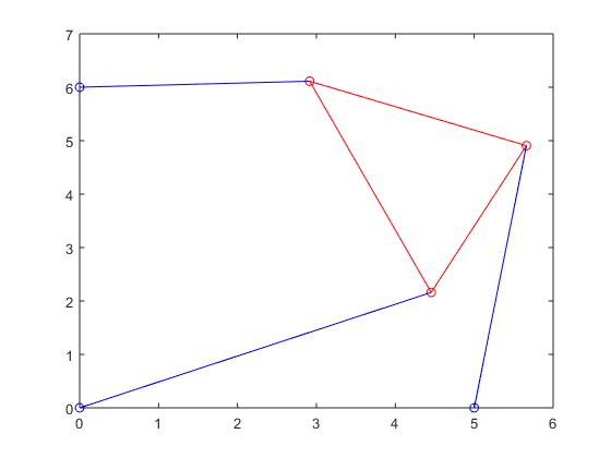
Stewart Platform when root was -0.9376:
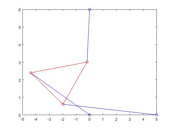
Stewart Platform when root was -0.0592:
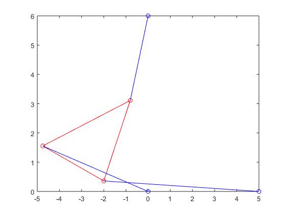
Stewart Platform when root was 1.1569:
Stewart Platform when root was 2.0495:
After repreating the same process for problem 4, except with with p2 set to 7.01 (7.01 because 7 did not produce the 6 required poses for this question), we were able to plot the function once more on the interval from [-π, π], which can be seen below:
 Once again throught the bisection method, we were able to use guessing and checking based on the graph produced above to determine the 6 poses. By using the plot above and the bisection method, we were able to generate the six distinct roots or poses: -0.6415, -0.4098, 0.0576, 0.4617, 0.9774, 2.5149. Once we obtained these poses (aka roots), we were again able to use the values to determine the values of x and y. The 6 new Stewart Platforms generated with the appropriate poses can be seen below, in respective order:
Stewart Platform when root was -0.6415:
Stewart Platform when root was -0.4098:
Stewart Platform when root was 0.0576:
Stewart Platform when root was 0.4617:
Stewart Platform when root was 0.9774:
Stewart Platform when root was 2.5149:
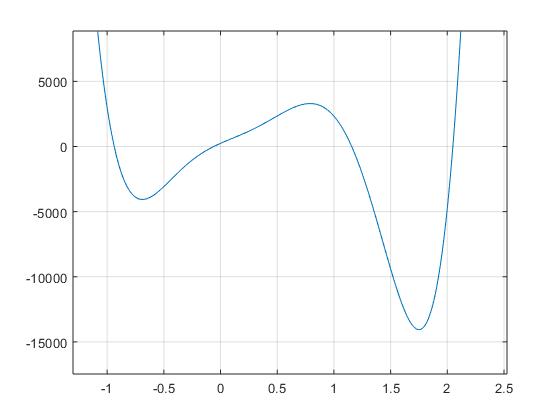
For the final task of this project, we were asked to find an appropriate strut length to result in two poses. In this problem, all other constant variables were held as the same, except for p2, which we essentially played around with until we produced a graph that indicated only 2 roots. In the end, we came to the result of p2 = 4, which resulted in only 2 poses/roots. The plot generated for the function f(θ) on the interval from [-π, π] can be seen again below, but for readability purposes, we zoomed in on the plot:
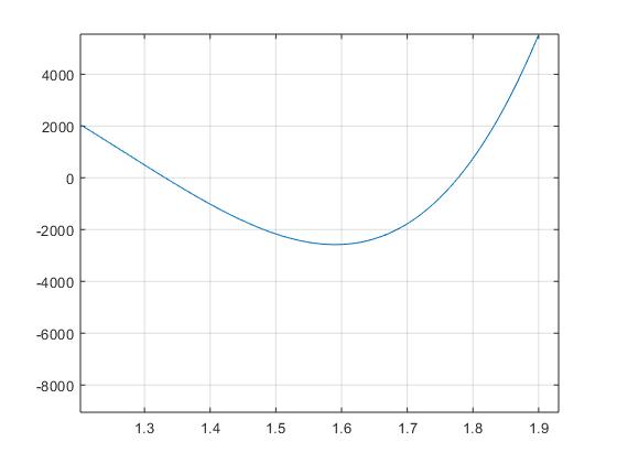 Finally, again through bisection method, we were able to derive the following 2 roots/poses for f(θ) when p2=4: 1.3500, 1.7700. Based on these values, we plotted the corresponding Stewart Platforms once more. These Stewart Platforms based on the roots above can be seen below:
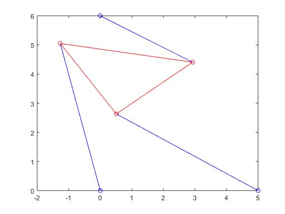
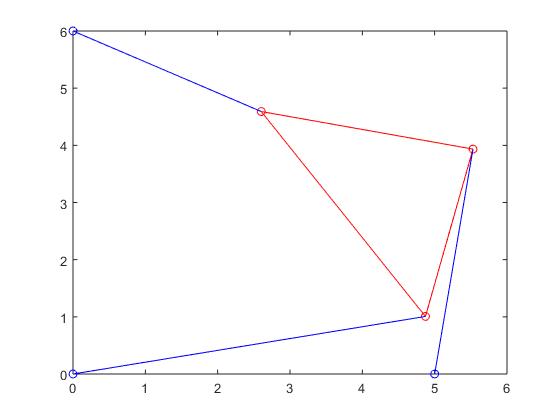
Stewart Platform when root was 1.3500:
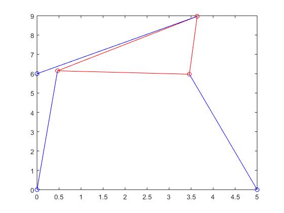
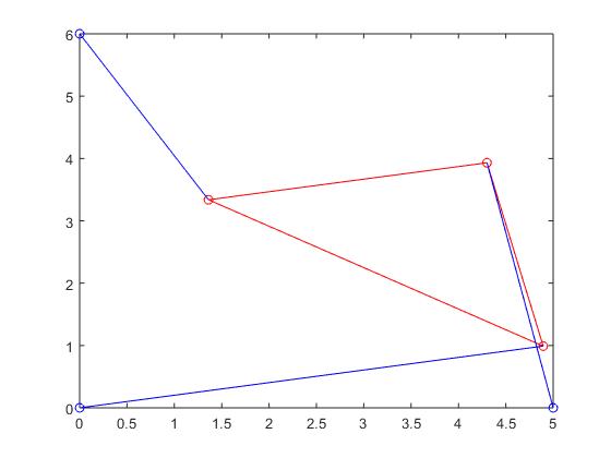
Stewart Platform when root was 1.7700:
In conclusion, we found that through the bisection method, we were able to generate a wide array of variable angles that could be used to generate the corrresponding x and y values in order to create Stewart Platforms supported by kinematics. It was also evident that the use of the bisection method was a quick way to solve for the roots of any given function that we implemented, while also being efficient. Although the bisection method may not always be the fastest algorithm (with a convegence rate of 0.5), it was appropriate to use in context of the problem as the bisection method always guarantees convergence to the root(s) (if existent). Future ways in which this project could be tackled could be by using the secant method, or even possibly the inverse quadratic interpolation method, both of which have their relative advantages and disadvantages.