In this project, we delve into Celestial Mechanics by simulating the effect of gravity on different objects given specific initial conditions. We will use Newton's law of universal gravitation, defined as: \[ \begin{align} F= \frac{gm_1m_2}{r^2}\\ \end{align} \] The law states that any two bodies in the universe attract to one another with a force \(F\). This force is directly proportional to the product of the masses, \(m_1\) and \(m_2\), and inversely proportional to the square of their distance, \(r\). For our evaluations, we will define \(g\), the gravitation constant, to be equal to \(1\). Then, looking at the force in terms of components: \[ \begin{align} (F_x,F_y) = (\frac{gm_1m_2}{x^2 + y^2}\frac{-x}{\sqrt{x^2+y^2}},\frac{gm_1m_2}{x^2 + y^2}\frac{-y}{\sqrt{x^2+y^2}}) \\ \end{align} \] Interpretting these components with regards to Newton's law of motion generates two second-order equations: \[ \begin{align} m_1x''= - \frac{gm_1m_2x}{(x^2 +y^2)^{3/2}} \\ m_2y''= - \frac{gm_1m_2y}{(x^2 +y^2)^{3/2}} \end{align} \] We can now introduce varaibles \(v_x = x'\) and \(v_y = y'\) to reduce our two second-order equations into four first-order equations: \[ \begin{align} x' & = v_x \\ v_x' & = -\frac{gm_2x}{(x^2 +y^2)^{3/2}} \\ y' & = v_y \\ v_y' & = -\frac{gm_2y}{(x^2 +y^2)^{3/2}} \end{align} \]
For the next three problems we will be applying Runge-Kutta Method of order four (RK4), rungekutta4step.m, to solve the system of first-order equations.
We will be solving a two-body problem for this step. The given masses are: \(m_1 = 0.03\), and \(m_2 = 0.3\). We are asked to plot the trajectories with intial conditions: \((x_1, y_1) = (2,2)\), \((x'_1, y'_1) = (0.2,-0.2)\) and \((x_2, y_2) = (0,0)\), \((x'_2, y'_2) = (-0.02,0.02)\). We use MATLAB program orbit2b.m to obtain the following results:

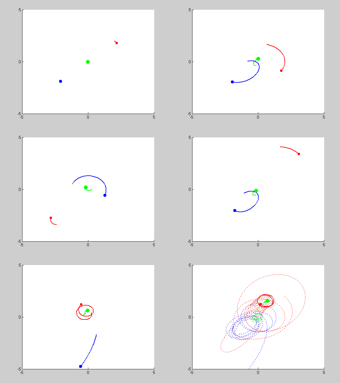
We will be solving a three-body problem for this step. The given masses are: \(m_1 = 0.03\), \(m_2 = 0.3\), and \(m_3 = 0.03\). We are asked to plot the trajectories with intial conditions: \((x_1, y_1) = (2,2)\), \((x'_1, y'_1) = (0.2,-0.2)\), \((x_2, y_2) = (0,0)\), \((x'_2, y'_2) = (0,0)\), and \((x_3, y_3) = (-2,2)\), \((x'_3, y'_3) = (-0.2,0.2)\). We use MATLAB program orbit3b.m to obtain the following results:

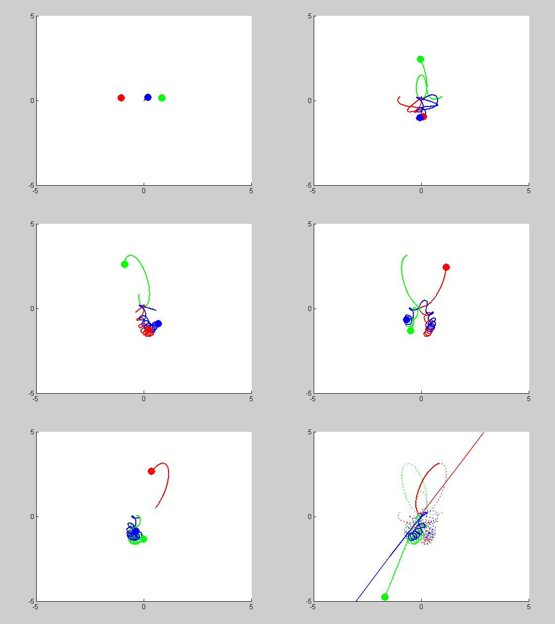
Changing the intial conditions of \(x'_1\) to \(0.20001\) results in the following case of sensitive dependence:

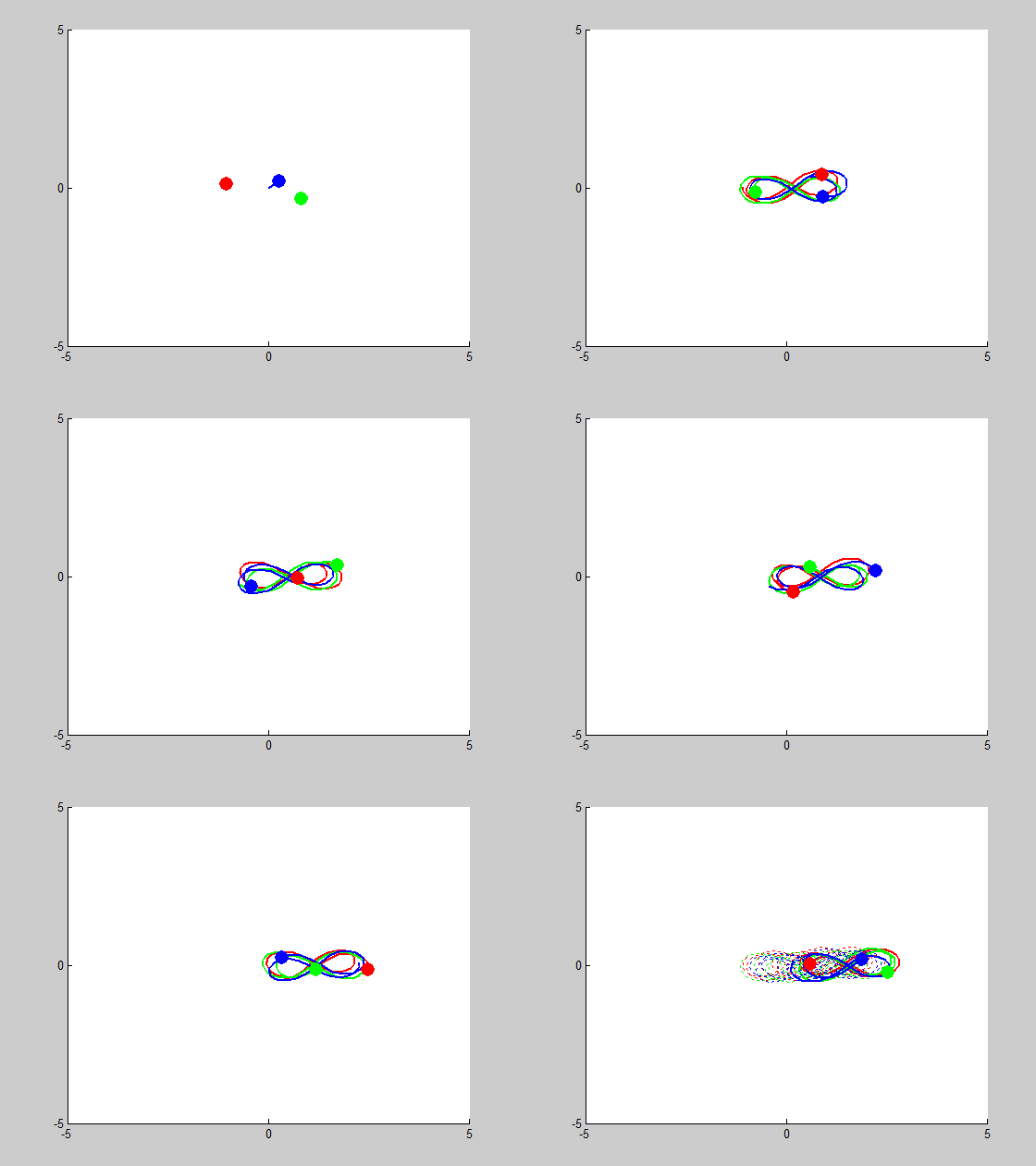
We will be solving a three-body problem for this step, only this time, a remarkable figure-eight orbit is expected to be achieved. The given masses are: \(m_1 = m_2 = m_3 = 1\). We are asked to plot the trajectories with intial conditions: \((x_1, y_1) = (-0.970,0.243)\), \((x'_1, y'_1) = (-0.466,-0.433)\), \((x_2, y_2) = (0,0)\), \((x'_2, y'_2) = (0,0)\), and \((x_3, y_3) = (0,0)\), \((x'_3, y'_3) = (-2x'_1,-2y'_1)\). We use MATLAB program orbit3b.m to obtain the following results:

We look into cases of sensitive dependence by changing \(x'_3\) by \(10^-k\) for \(1\leq k \leq5\). It proved remarkably stable in the \(k=3, k=4\) and \(k=5\) cases, essentially no disruption is noticeable. At \(k=2\), some slight drifting from orbit to orbit can be observed, and when \(k=1\) the entire system drifts to the right, but in both of these cases the overall figure-eight pattern of motion remains the same.
Figure 8 (\(k^{-5}\) error):

Figure 8 (\(k^{-2}\) error):

Figure 8 (\(k^{-1}\) error):

Chaotic but controlled behaviour:

Chaotic behavior followed by near-singularity:
