Project 1: Kinematics of the Stewart Platform
Team members: Aidan Curran, Varis Nijat, Faysal Shaikh
Contents
Background
A Stewart platform consists of six variable length struts, or prismatic joints, supporting a payload. Prismatic joints operate by changing the length of the strut, usually pneumatically or hydraulically. As a six-degree-of-freedom robot, the Stewart platform can be placed at any point and inclination in three-dimensional space that is within its reach.
Our goal is to solve the forward kinematics problem, namely, to find  ,
,  , and
, and  , given
  ,
,  , and
, and  .
.
Part 1-- Write (and test) the function.
Write a MATLAB function file for  . The parameters
  ,
,  ,
,  ,
,  ,
,  , (implied
  ,)
,)  ,
,  are fixed constants, and the strut lengths
  ,
,  ,
,  will be known for a given pose.
To test our code, substituting  should show
  .
.
%test case 1: pi/4
theta_1=pi*(1/4);
test_1=f(theta_1)


%test case 2: -pi/4
theta_2=-1*pi*(1/4);
test_2=f(theta_2)
test_1 =

  -4.5475e-13


test_2 =

  -4.5475e-13
As we can see,  . Thus, our function seems to be working correctly.
Part 2-- Plot the function.
Plot  on
on ![$[-\pi,\pi]$](full_report_eq04277113708218156659.png) . You may use the @ symbol as described in Appendix B.5 to assign a function handle to your function file in the plotting command. You may also need to precede arithmetic operations with the "." character to vectorize the operations, as explained in Appendix B.2. As a check of your work, there should be roots at
. You may use the @ symbol as described in Appendix B.5 to assign a function handle to your function file in the plotting command. You may also need to precede arithmetic operations with the "." character to vectorize the operations, as explained in Appendix B.2. As a check of your work, there should be roots at  .
.
%plot vectorized function f_2(theta) on [-pi,pi]


%plot using fplot
fplot(@(theta) f_2(theta),[-1*pi,pi])


%hold to continue plotting-- plot x=0
hold on

fplot(0)


%end plotting
hold off


%set x-axis limits
xlim([-pi pi])


%calculate value of pi/4
val=pi/4
val =

    0.7854
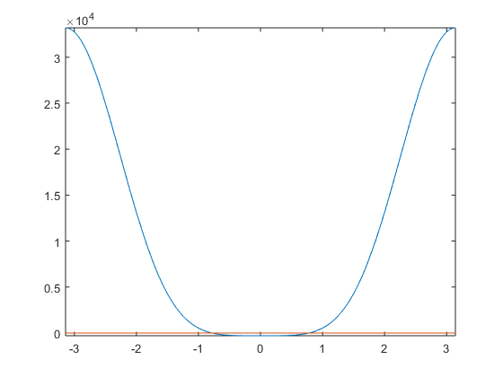
Looking at "val" above, the value of  , the picture above seems to depict roots at
  ; the function appears to be correct.
Part 3-- Reproduce Figure 1.15.
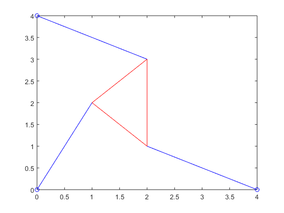
Reproduce Figure 1.15 from Reality Check 1.
Reproduce Figure 1.15 (a):
%strut beginning positions
x0=0; %implied-- never included in book figures/equations
y0=0; %implied-- never included in book figures/equations

x1=4;
y1=0; %implied-- never included in book figures/equations

x2=0;
y2=4;


%stewart platform vertex points
x=1;
y=2;

u1=x;
v1=y;

u2=2;
v2=3;

u3=2;
v3=1;


%plot red triangle (planar Stewart platform) and hold
plot([u1 u2 u3 u1],[v1 v2 v3 v1],'r');

hold on


%plot strut beginning points
plot([x0,x1,x2],[y0,y1,y2],'bo')


%plot strut length lines
plot([x0 u1],[y0 v1],'b')
plot([x1,u3],[y1,v3],'b')
plot([x2 u2],[y2 v2],'b')


%complete plot
hold off
Reproduce Figure 1.15 (b):
%strut beginning positions
x0=0; %implied-- never included in book figures/equations
y0=0; %implied-- never included in book figures/equations

x1=4;
y1=0; %implied-- never included in book figures/equations

x2=0;
y2=4;


%stewart platform vertex points
x=2;
y=1;

u1=x;
v1=y;

u2=1;
v2=2;

u3=3;
v3=2;


%plot red triangle (planar Stewart platform) and hold
plot([u1 u2 u3 u1],[v1 v2 v3 v1],'r');

hold on


%plot strut beginning points
plot([x0,x1,x2],[y0,y1,y2],'bo')


%plot strut length lines
plot([x0 u1],[y0 v1],'b')
plot([x1,u3],[y1,v3],'b')
plot([x2 u2],[y2 v2],'b')


%complete plot
hold off
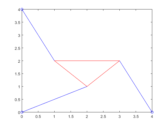
Figures 1.15 (a) and (b) seem to be reproduced reliably above.
Part 4-- Solve (with given parameters).
 ,
,  ,
,  ,
,  ,
,  ,
,  ,
,  .
.
First, plot the function.
%plotting
ezplot(@f_4,[-pi,pi])
hold on
plot([-pi,pi],[0,0])
hold off
Warning: Function failed to evaluate on
array inputs; vectorizing the function may
speed up its evaluation and avoid the need
to loop over array elements.
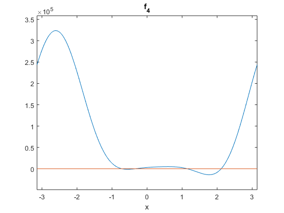
The function appears to have roots near -0.75, -0.4, 1.2, and 2.1. Utilize the fzero equation solver to determine the roots of the function.
%root-finding (approximating theta)
theta_1=fzero(@f_4,-0.75)
theta_2=fzero(@f_4,-0.4)
theta_3=fzero(@f_4,1.2)
theta_4=fzero(@f_4,2.1)
theta_1 =

   -0.7208


theta_2 =

   -0.3310


theta_3 =

    1.1437


theta_4 =

    2.1159
Using the above values for  , determine the appropriate values of
  and
and  . For this purpose, created xy_solv_4.m.
%equation solver (find x and y from theta)
xy_p4_1=xy_solv_4(theta_1)
xy_p4_2=xy_solv_4(theta_2)
xy_p4_3=xy_solv_4(theta_3)
xy_p4_4=xy_solv_4(theta_4)
xy_p4_1 =

   -1.3784    4.8063


xy_p4_2 =

   -0.9147    4.9156


xy_p4_3 =

    4.4818    2.2167


xy_p4_4 =

    4.5718    2.0244
Using the above values for  and
and  , solve the inverse kinematics problem of the planar Stewart platform (by finding
  ,
,  , and
, and  , given
  ,
,  , and
, and  ) to verify that strut lengths are indeed as specific at the beginning of the problem. For this purpose, created reverse_solv_4.m.
%equation solver (find p1, p2, p3 from x, y, theta)
p_vec_p4_1=reverse_solv_4(xy_p4_1(1),xy_p4_1(2),theta_1)
p_vec_p4_2=reverse_solv_4(xy_p4_2(1),xy_p4_2(2),theta_2)
p_vec_p4_3=reverse_solv_4(xy_p4_3(1),xy_p4_3(2),theta_3)
p_vec_p4_4=reverse_solv_4(xy_p4_4(1),xy_p4_4(2),theta_4)
p_vec_p4_1 =

    5.0000    5.0000    3.0000


p_vec_p4_2 =

    5.0000    5.0000    3.0000


p_vec_p4_3 =

    5.0000    5.0000    3.0000


p_vec_p4_4 =

    5.0000    5.0000    3.0000
As seen above, the solutions found seem to be in accordance with the initially-specified values for strut-lengths. The solution is correct!
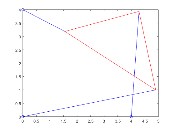
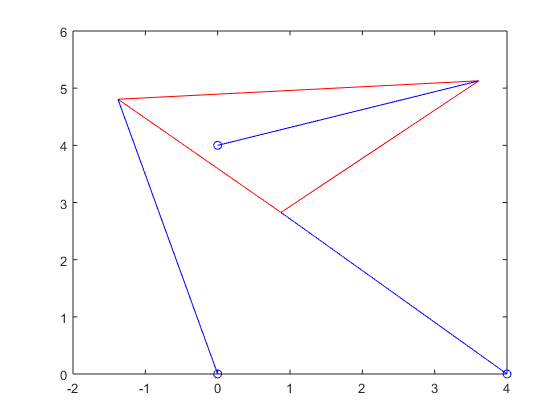
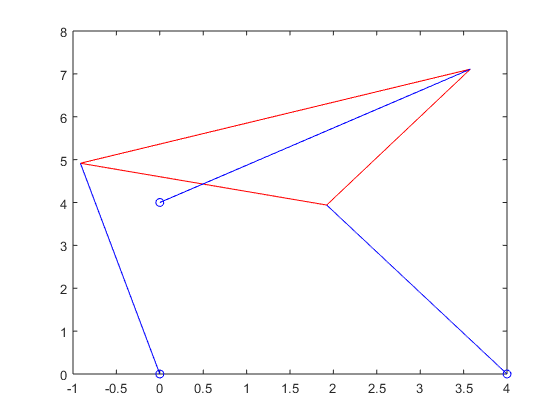
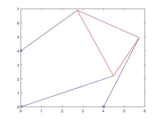
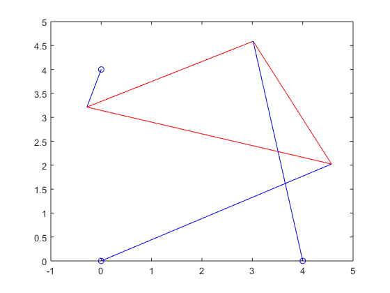
The exercise also requires plotting the positions of the Stewart platform. To accomplish this task, Stewart_plot.m was created.
Finally, here are the plotted positions of the Stewart platform:
Finally, here are the plotted positions of the Stewart platform:
Stewart_plot(xy_p4_1(1),xy_p4_1(2),theta_1,p_vec_p4_1(1),p_vec_p4_1(2),p_vec_p4_1(3))
Stewart_plot(xy_p4_2(1),xy_p4_2(2),theta_2,p_vec_p4_2(1),p_vec_p4_2(2),p_vec_p4_2(3))
Stewart_plot(xy_p4_3(1),xy_p4_3(2),theta_3,p_vec_p4_3(1),p_vec_p4_3(2),p_vec_p4_3(3))
Stewart_plot(xy_p4_4(1),xy_p4_4(2),theta_4,p_vec_p4_4(1),p_vec_p4_4(2),p_vec_p4_4(3))
Part 5-- Resolve Part 4 (with a minor modification).
Same parameters as Part 4, but with  .
.
First, plot the function.
%plotting
ezplot(@f_5,[-pi,pi])
hold on
plot([-pi,pi],[0,0])
hold off
Warning: Function failed to evaluate on
array inputs; vectorizing the function may
speed up its evaluation and avoid the need
to loop over array elements.
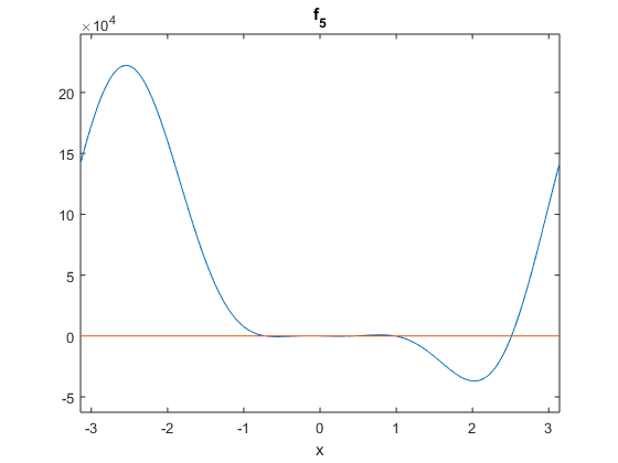
Things are still not as clear with this picture, so let's look at it from closer to the x-axis.
%plotting
ezplot(@f_5,[-pi,pi])
hold on
plot([-pi,pi],[0,0])
hold off


%setting y-axis limits
ylim([-1 1])
Warning: Function failed to evaluate on
array inputs; vectorizing the function may
speed up its evaluation and avoid the need
to loop over array elements.
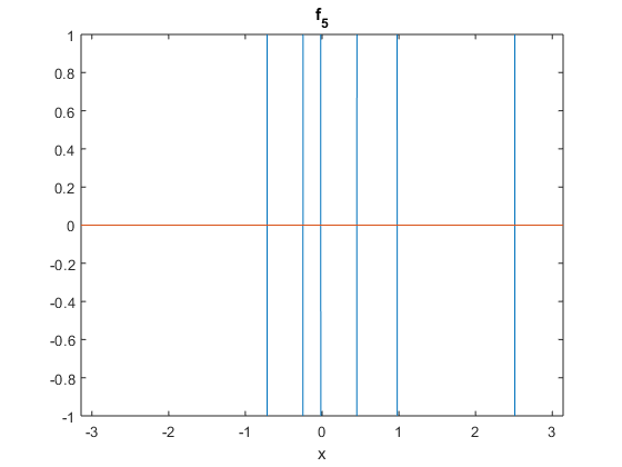
The function appears to have roots near -0.8, -0.4, -0.1, 0.5, 1, and 2.5. This is 6 poses, as described in the question, so we are on the right track. Utilize the fzero equation solver to determine the roots of the function.
%root-finding (approximating theta)
theta_p5_1=fzero(@f_5,-0.8)
theta_p5_2=fzero(@f_5,-0.4)
theta_p5_3=fzero(@f_5,-0.1)
theta_p5_4=fzero(@f_5,0.5)
theta_p5_5=fzero(@f_5,1)
theta_p5_6=fzero(@f_5,2.5)
theta_p5_1 =

   -0.7164


theta_p5_2 =

   -0.2490


theta_p5_3 =

   -0.0174


theta_p5_4 =

    0.4532


theta_p5_5 =

    0.9782


theta_p5_6 =

    2.5117
Using the above values for  , determine the appropriate values of
  and
and  . For this purpose, created xy_solv_5.m.
%equation solver (find x and y from theta)
xy_p5_1=xy_solv_5(theta_p5_1)
xy_p5_2=xy_solv_5(theta_p5_2)
xy_p5_3=xy_solv_5(theta_p5_3)
xy_p5_4=xy_solv_5(theta_p5_4)
xy_p5_5=xy_solv_5(theta_p5_5)
xy_p5_6=xy_solv_5(theta_p5_6)
xy_p5_1 =

   -4.2035    2.7074


xy_p5_2 =

   -4.8783    1.0963


xy_p5_3 =

   -4.9469    0.7271


xy_p5_4 =

   -0.8100    4.9340


xy_p5_5 =

    2.3355    4.4210


xy_p5_6 =

    3.2329    3.8142
Using the above values for  and
and  , solve the inverse kinematics problem of the planar Stewart platform (by finding
  ,
,  , and
, and  , given
  ,
,  , and
, and  ) to verify that strut lengths are indeed as specific at the beginning of the problem. For this purpose, created reverse_solv_5.m.
%equation solver (find p1, p2, p3 from x, y, theta)
p_vec_p5_1=reverse_solv_5(xy_p5_1(1),xy_p5_1(2),theta_p5_1)
p_vec_p5_2=reverse_solv_5(xy_p5_2(1),xy_p5_2(2),theta_p5_2)
p_vec_p5_3=reverse_solv_5(xy_p5_3(1),xy_p5_3(2),theta_p5_3)
p_vec_p5_4=reverse_solv_5(xy_p5_4(1),xy_p5_4(2),theta_p5_4)
p_vec_p5_5=reverse_solv_5(xy_p5_5(1),xy_p5_5(2),theta_p5_5)
p_vec_p5_6=reverse_solv_5(xy_p5_6(1),xy_p5_6(2),theta_p5_6)
p_vec_p5_1 =

    5.0000    6.9800    3.0000


p_vec_p5_2 =

    5.0000    6.9800    3.0000


p_vec_p5_3 =

    5.0000    6.9800    3.0000


p_vec_p5_4 =

    5.0000    6.9800    3.0000


p_vec_p5_5 =

    5.0000    6.9800    3.0000


p_vec_p5_6 =

    5.0000    6.9800    3.0000
As seen above, the solutions found seem to be in accordance with the initially-specified values for strut-lengths. The solution is correct!
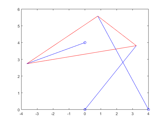
Finally, here are the plotted positions of the Stewart platform:
Stewart_plot(xy_p5_1(1),xy_p5_1(2),theta_p5_1,p_vec_p5_1(1),p_vec_p5_1(2),p_vec_p5_1(3))
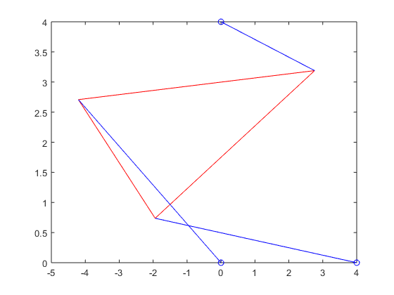
Stewart_plot(xy_p5_2(1),xy_p5_2(2),theta_p5_2,p_vec_p5_2(1),p_vec_p5_2(2),p_vec_p5_2(3))
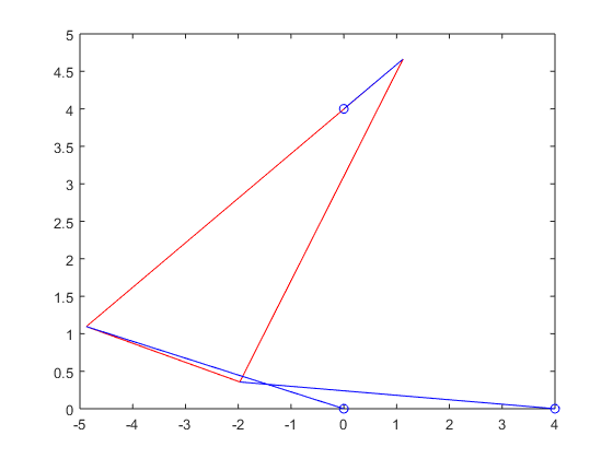
Stewart_plot(xy_p5_3(1),xy_p5_3(2),theta_p5_3,p_vec_p5_3(1),p_vec_p5_3(2),p_vec_p5_3(3))
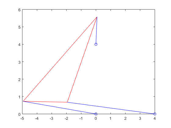
Stewart_plot(xy_p5_4(1),xy_p5_4(2),theta_p5_4,p_vec_p5_4(1),p_vec_p5_4(2),p_vec_p5_4(3))
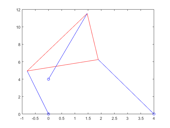
Stewart_plot(xy_p5_5(1),xy_p5_5(2),theta_p5_5,p_vec_p5_5(1),p_vec_p5_5(2),p_vec_p5_5(3))
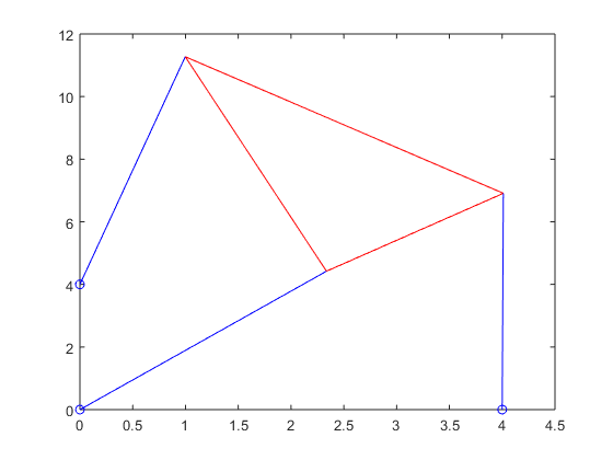
Stewart_plot(xy_p5_6(1),xy_p5_6(2),theta_p5_6,p_vec_p5_6(1),p_vec_p5_6(2),p_vec_p5_6(3))
Part 6-- Solve the inverse kinematics problem, using parameters from Part 4, for only 2 poses.
Find a strut length p2, with the rest of the parameters as in Step 4, for which there are only two poses
Following trial and error, a value for  was eventually found that leads to only 2 positions of the Stewart platform (2 different values of
  ):
):
%plotting
ezplot(@f_6,[-pi,pi])
hold on
plot([-pi,pi],[0,0])
hold off
Warning: Function failed to evaluate on
array inputs; vectorizing the function may
speed up its evaluation and avoid the need
to loop over array elements.
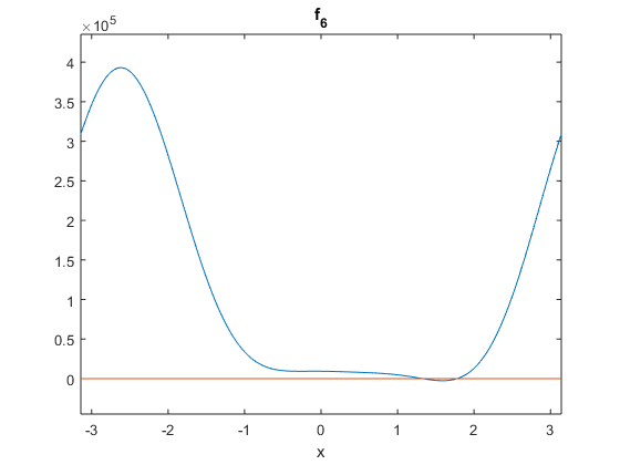
As the above function is seen to dip below the x-acis between 1 and 2 and return after 2, it is necessarily the case that exactly 2 roots exist within this viewing window.
theta_p6_1=fzero(@f_6,1.3)
theta_p6_2=fzero(@f_6,1.7)
theta_p6_1 =

    1.3316


theta_p6_2 =

    1.7775
Using the above values for  , determine the appropriate values of
  and
and  . For this purpose, created xy_solv_6.m.
%equation solver (find x and y from theta)xy_p6_1=xy_solv_6(theta_p6_1)
xy_p6_1=xy_solv_6(theta_p6_1)
xy_p6_2=xy_solv_6(theta_p6_2)
xy_p6_1 =

    4.8907    1.0399


xy_p6_2 =

    4.8992    0.9992
%equation solver (find p1, p2, p3 from x, y, theta)
p_vec_p6_1=reverse_solv_6(xy_p6_1(1),xy_p6_1(2),theta_p6_1)
p_vec_p6_2=reverse_solv_6(xy_p6_2(1),xy_p6_2(2),theta_p6_2)
p_vec_p6_1 =

    5.0000    4.0000    3.0000


p_vec_p6_2 =

    5.0000    4.0000    3.0000
As seen above, the solutions found seem to be in accordance with the initially-specified values for strut-lengths. The solution is correct!
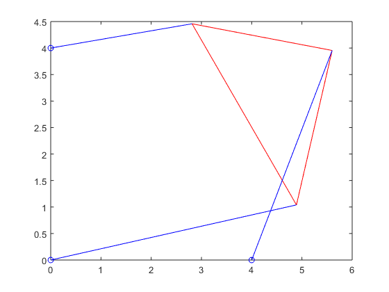
Finally, here are the plotted positions of the Stewart platform:
Stewart_plot(xy_p6_1(1),xy_p6_1(2),theta_p6_1,p_vec_p6_1(1),p_vec_p6_1(2),p_vec_p6_1(3))
Stewart_plot(xy_p6_2(1),xy_p6_2(2),theta_p6_2,p_vec_p6_2(1),p_vec_p6_2(2),p_vec_p6_2(3))
