Due to our abilities to measure things at best discretely, given some sampled data, we may want to reconstruct what the continous form of the function may have been. Then
from there, we could utilize the information provided from that form of the data to draw further results. The tools needed for this job are discrete transforms.
In our investigation here, the particular transform used will be the modified discrete cosine transform (MDCT for short). This transform provides the right coefficients that would
be used to best approximate the signal in terms of continous cosines. We get these coefficients by multiplying our input data (which tends to be a signal) with a \(n \times 2n\) matrix M where:
\[ M_{ij} = \sqrt{\frac{2}{n}}\cos{\frac{(2i+1)(j+\frac{n+1}{2})\pi}{2n}}\] We also note that both \(i,j\) start at \(0\) instead of the conventional \(1\).
In our demonstration, we will investigate the practical use ofthe MDCT with audio compression techniques. When transporting audio, there is a restriction on the space at
which it can be sent without issues arising. So there must be a technique that compresses the data in filesize in such a way that it can be sent cleanly, without a big tradeoff of the
actual quality. An example is an audio engineer or a music producer may create several audio pieces that are each about 40 MB .wav file, and they wish to place all these
on a CD, which on average can only hold 80 MB. This is precisely what the MDCT will be used for; to compress the signal and then decode the signal so that it's compressed form is near similar to its original
form.
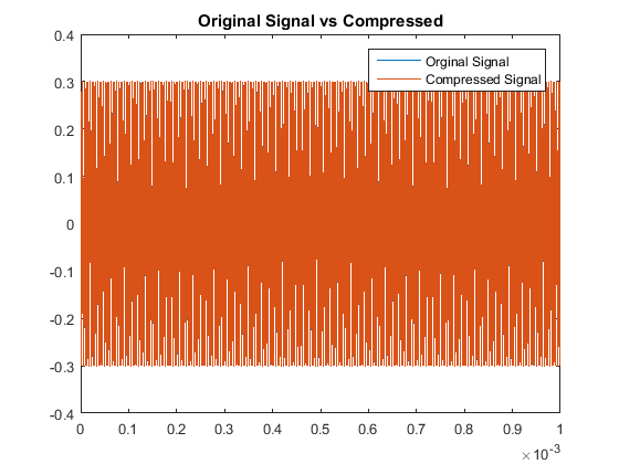
We utilize a bare-bones audio compression algorithm here to investigate pure tones of \(64f\) Hz for small \(f\in \mathbb{Z}\), that
can be represented as sampled data from a cosine function. We test even an odd multiples of 64 to test our algorithm's accuracy. Comparing auditory sounds we have:
\(f\) Multiple
Original Sounds
Compressed Sounds
\(1\)
\(2\)
\(3\)
\(4\)
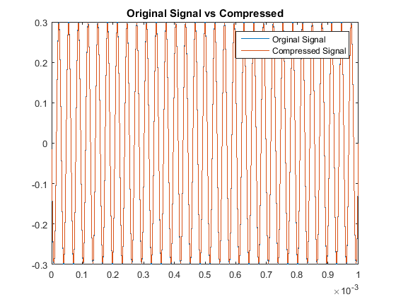
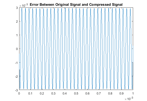
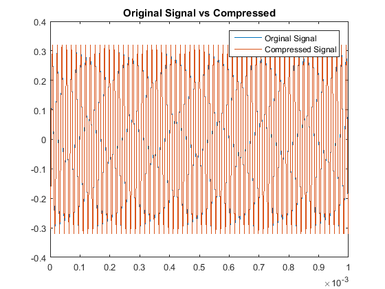
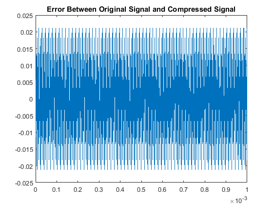
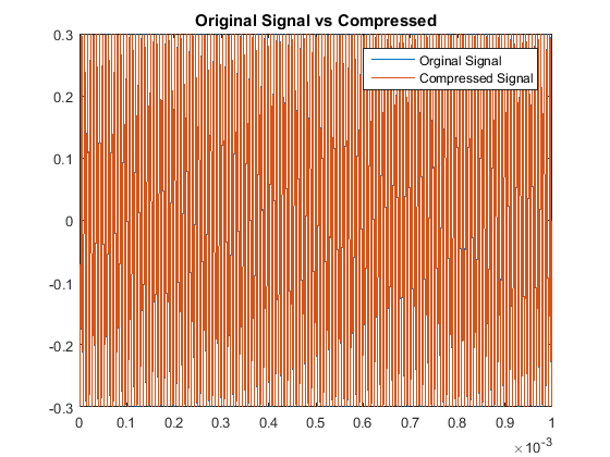
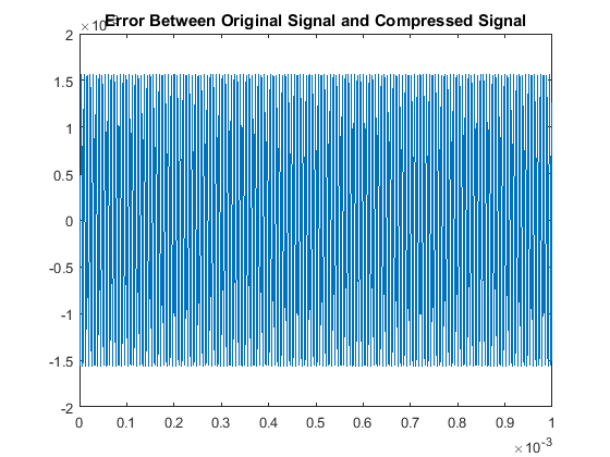
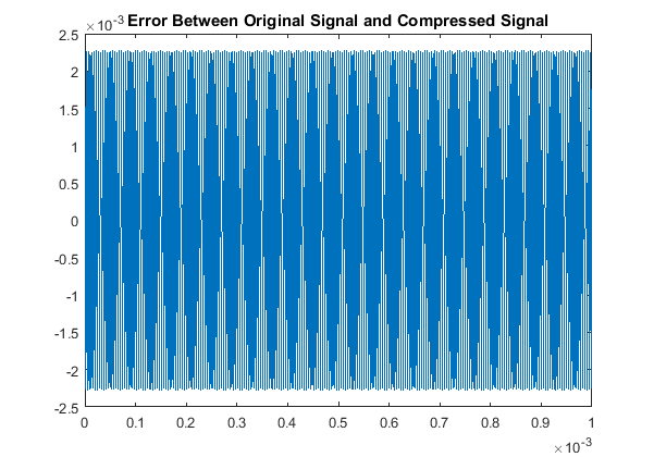
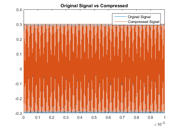
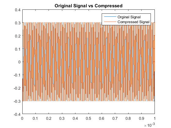
Then when comparing the acutal signals from a quantitative point of view, our results are:
\(f\) Multiple
Signal Comparisons
Signal Error
RMSE
\(1\)
\(0.0021\)
\(2\)
\(0.0095\)
\(3\)
\(0.0017\)
\(4\)
\(0.0091\)
\(5\)
\(0.0011\)
\(6\)
\(0.0097\)
\(7\)
\(0.0016\)
\(8\)
\(0.0095\)
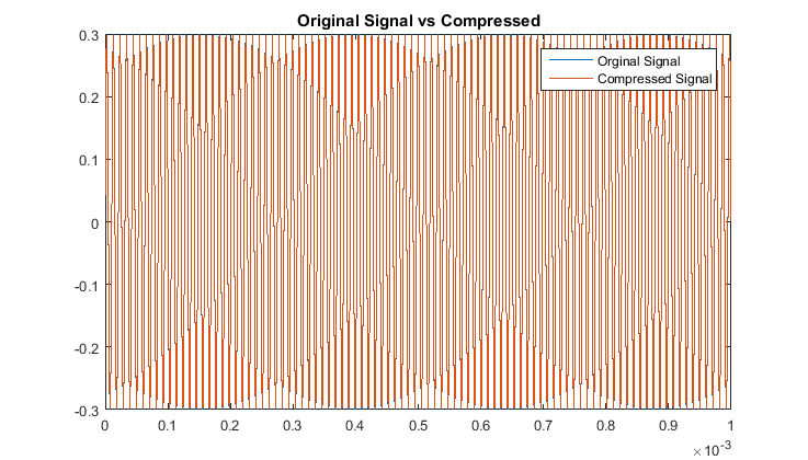
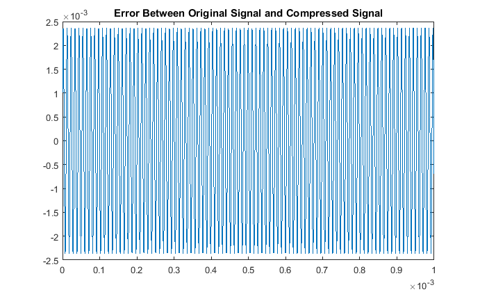
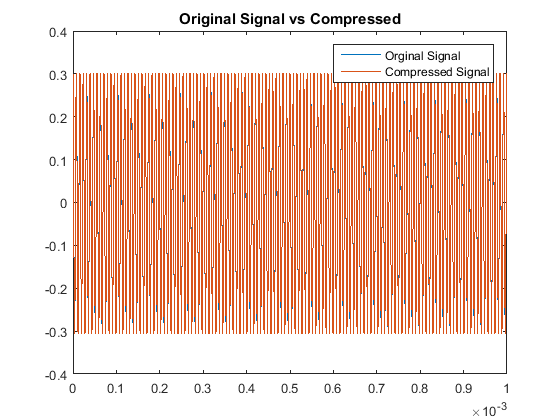
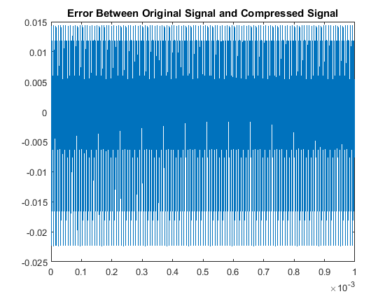
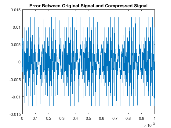
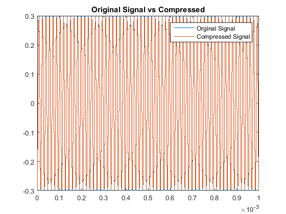
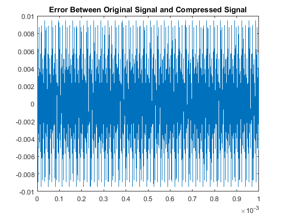
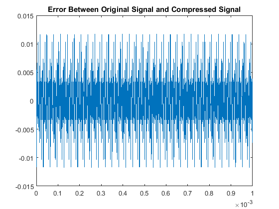
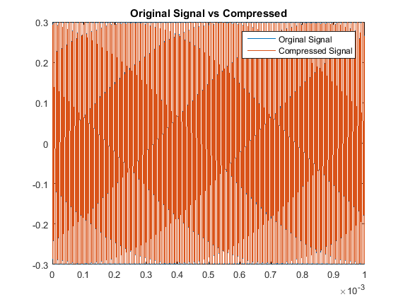
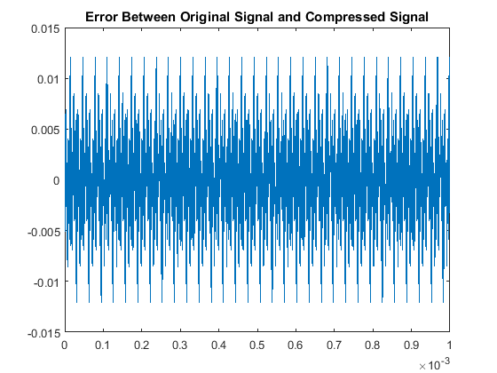
With respect to the RMSE of that compares the original and compressed signals, there is a notably consistent spike in the accuracy, or lack thereof, for even multiples
of these pure tones in comparison to the odd multiples. This may be due to the process of rounding the MDCT vector components when they are quantized. Additionally we note
that all the continous modes of the odd-multiple tones have some of the same roots, while all the even multiples are all shifted in their respective roots. That inconsistency
will cause an increase-in-error issue as you consider the not-so-nice shift in sampled input data as all these are suppose to have the same time discretization. The code used here was
signalcompare1 and simplecodec
In an attempt to improve the accuracy so that our even multiples of pure tones can be accurately compressed, we componentwise-scale
our input data with a sampled windowing function \(h\) where: \[h_j = \sqrt{2}\sin{\frac{(j-\frac{1}{2})\pi}{2n}} \]. We know this will still keep our algorithm consistent because of
the following observation.
By following the notation in the book, let the vector \(h= [h_1,h_2,h_3,h_4]\) where each \(h_i\) is a \(\frac{n}{2} {}\) long vector. Then for our \(Z_1\) vector we have that each
section can be now written as \(x_ih_i\) where this multiplication is component-wise. Since our \(Z_2\) vector is an overlapping vector with \(Z_1\), then we know that
\[Z_2 = \left[\begin{array}{c}
x_3h_3\\
x_4h_4\\
x_5h_1\\
x_6h_2 \end{array} \right]\] Now by moving on we pay particular close attention to the last two
and the first two sections of our \(NMZ_1\) and \(NMZ_2\) vectors. we note that respectively these are:
\[(NMZ_1)_{3,4} = \left[\begin{array}{c}
x_3h_3+Rx_4h_4\\
Rx_3h_3+x_4h_4\\
\end{array} \right],
(NMZ_2)_{1,2} = \left[\begin{array}{c}
x_3h_3-Rx_4h_4\\
-Rx_3h_3+x_4h_4\\
\end{array} \right]\]
From there we can see that:
\[ \frac{1}{2}\left((NMZ_1)_{3,4}+(NMZ_2)_{1,2} \right)= \left[ \begin{array}{c}
x_3h_3\\
x_4h_4 \end{array} \right] \]
By setting \(x_ih_i=x_i '\), we can see that the equations in the book still hold; and thus, the decoding of the signal
is still consistent when scaling our input data.
We note that this code is simply a modification of
the latter half of previous code used. When testing our windowing function we notice the auditory output, we note that the original sounds stay the same:
\(f\) Multiple
Original Sounds
Compressed Sounds
\(1\)
\(2\)
\(3\)
\(4\)
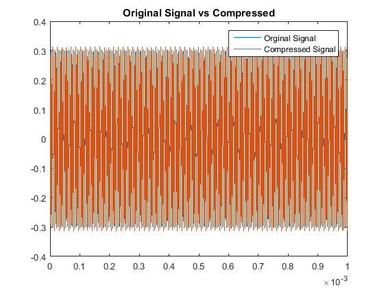
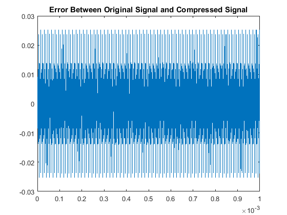
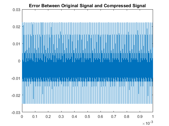
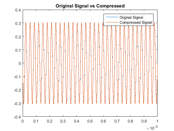
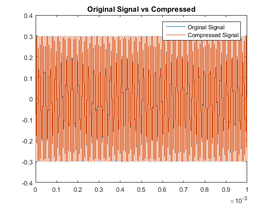
In a similar fashion as section I, we see our quantitative results are:
\(f\) Multiple
Signal Comparisons
Signal Error
RMSE
\(1\)
\(0.0045\)
\(2\)
\(0.0033\)
\(3\)
\(0.0043\)
\(4\)
\(0.0011\)
\(5\)
\(0.0043\)
\(6\)
\(0.0014\)
\(7\)
\(0.0048\)
\(8\)
\(0.0026\)
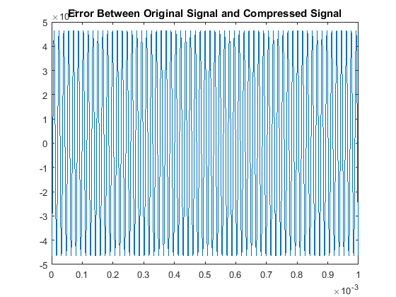
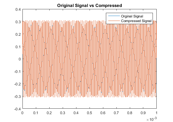
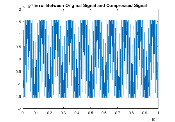
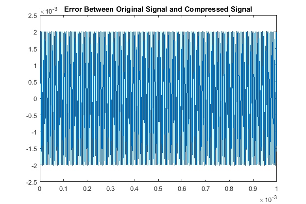
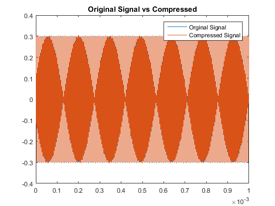
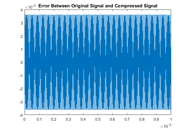
So although this scaling process made our odd multiples not as accurate as our original algorithm,
we have drastically improved our decoding accuracy for the even multiples. This is the other code used.
Here we investigate more complicated tones; in our case we will look at a certain type
of chord. The chord will generate by adding various pure tones. The chord that will be analyzed here will be a
third chord, so the frequency ratio is a 5:4 ratio. This chord sounds like:
We note when seeing how the the number of bits used affects the accuracy
we find out that:
Bits
RMSE
Compressed Sound
\(2\)
\(.0162\)
\(3\)
\(.0082\)
\(4\)
\(.0049\)
\(5\)
\(.0021\)
\(6\)
\(.0012\)
\(7\)
\(7.6247*10^{-4}\)
\(8\)
\(4.2358*10^{-4}\)
So we see that as we increase the amount of bits used, there does seem to be a general increase in accuracy. The code used is here
Here, we actually decide to try our techniques on an audio sample from the movie Sound of Music . We test to see what happens when we change
the bits used, as well if we use our window-scaling or not. The original sample is:
Our results are below:
Bits
Windowed Sound
Windowed RMSE
Non-Windowed Sound
Non-Windowed RMSE
\(2\)
\(0.0124\)
\(0.0148\)
\(3\)
\(0.0066\)
\(0.0090\)
\(7\)
\(6.0616*10^{-4}\)
\(8.9001*10^{-4}\)
\(8\)
\(3.3541*10^{-4}\)
\(4.5884*10^{-4}\)
Due to inconsistency of the RMSE, it seems that the windowing and non-windowing techniques seems similar in nature. We also notice that once again, we have that increasing
the bits used increases audio compression accuracy. This is the code here