Hannah Andrada, Robert Argus, Mezel Smith
In the 1940s, the Tacoma Narrows Bridge dealt with high winds, which caused torsional shifting. That shifting occurred for 45 minutes prior to its historical collapse into the Puget Sound. In our investigation, we utilized the mathematical models developed by McKenna and Tuama(2011):
\(\begin{align*} y'' &= -dy'-\frac{K}{ma}\left(e^{a(y-l\sin(\theta))}+e^{a(y+l\sin(\theta))}-2 \right)\\ \theta '' &= -d\theta ' +\frac{3\cos(\theta)}{l}\frac{K}{ma} \left( e^{a(y-l\sin(\theta))}+e^{a(y+l\sin(\theta))} \right) \end{align*}\)
Where:
\(\begin{align*}
a &= \text{Hooke's Law nonlinearity coefficient}\\
d &= \text{damping coefficient}\\
l &= \text{width of the bridge}\\
W &= \text{wind speed}\\
K &= \text{spring constant}\\
\omega &= \text{angular frequency of bridge}
\end{align*}\)
From there we perform experimental, mathematical analysis based upon the model to gain further insight as to what happened, what may have caused the collapse, and what things could have prevented it.
We first acknowledge that the models shown above cannot be solved analytically due to the complex, nonlinear nature of composite functions involved in the differential equations. This results in us solving it numerically. In particular, we utilized two numerical approximations: trapezoidal and a fourth order Runga-Kutta Method. To get some intuition into our model, we edit a program (see Animation Code) that will output an animation of what the bridge would do, given some initial conditions set on the bridge. When we have the initial angular displacement (in radians) be \(0.001\), and the wind speed \(W = 80\frac{\text{km}}{\text{h}}\), we see the bridge becomes torsionally unstable after about approximately a few hours:
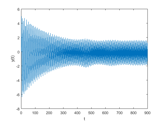
When actually seeing how the vertical displacement \( y(t) \) and the central angular displacement \( \theta(t) \) temporally evolve, we see that the accuracy of the animation will depend upon the accuracy of our numerical approximation of these functions. In particular, when comparing the trapezoidal and RK4 Methods we do see notable differences:
| State Variable | Trapezoidal Approximations | RK4 Approximations |
| \(y(t)\) | 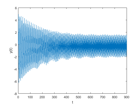 |
 |
| \(\theta(t)\) | 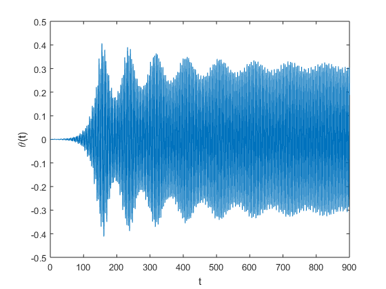 |
 |
We are already aware that the RK4 is a higher-order method than trapezoidal. Therefore we should expect our RK4 approximation to be more accurate. Additionally we notice that although the vertical displacement is relatively similar, we see that the moment of catastrophy with respect to the Angular displacement, occurs two hours later with the RK4 approximation than it does with the trapezoidal approximation. We also note that we used the same Animation Code when getting these plots; we just alternate between using the trapstep function and the rk4step function for the approximation.
Based upon intuition that the wind speed affects torisonal stability, we now investigate alternating the wind speed from before. So we are given that in the case of this model, torisonal stability should occur at \(W = 50\frac{\text{km}}{\text{h}}\). To verify this, we numerically approximate the angular displacement using our most accurate method at hand, RK4, resulting in the following:
which does indeed, verify the torsional stability.
| \(10^{-i}\) | EMF |
| 3 | 19.0153 |
| 4 | 18.8935 |
| 5 | 18.8922 |
| 6 | 18.8922 |
| 7 | 18.8922 |
| 8 | 18.8922 |
| 9 | 18.8922 |
| 10 | 18.8922 |
| 11 | 18.8920 |
| 12 | 18.8931 |
| 13 | 18.8932 |
| 14 | 18.6625 |
| 15 | 19.4819 |
| 16 | 8.3452 |
| Average | Standard Deviation |
| 18.1736 | 2.8342 |
The minimum wind speed W for which a small disturbance \(\theta(0) = 10^{-3}\) has a magnification factor of 100 or more is approximately 128.6651 \(\frac{km}{hr}\) in which the observed error magnification factor was found to be 100.0003. We initially observed a sensitive dependence of the error magification factor for values ranging between 128 and 128.7, which allowed us to further dial in the aforementioned windspeed. A consistent magnification factor can in fact be defined for the W. We determined the first magnification factor using the following code here and statistics were gathered using the following here.
An implementation of a method for computing the minimum wind speed to within \(0.5 \times 10^{-3}\frac{km}{hr}\) is given here.Experimenting with different wind speeds we obtain the plots below. From this figures we can discern that extremely small initial angles eventually grow to catastrophic size.
| W | \(\theta(t)\) | W | \(\theta(t)\) | W | \(\theta(t)\) |
| 55 | 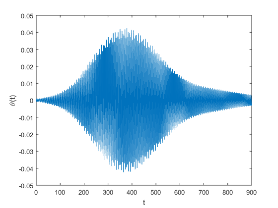 |
57.5 | 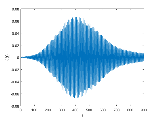 |
60 | 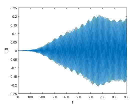 |
| 65 | 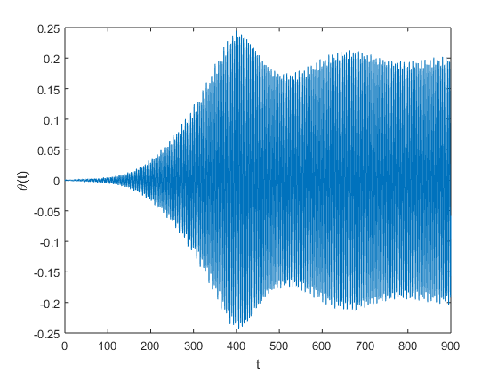 |
100 | 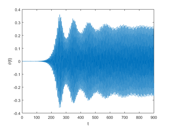 |
129 |  |
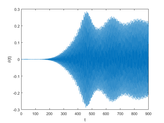
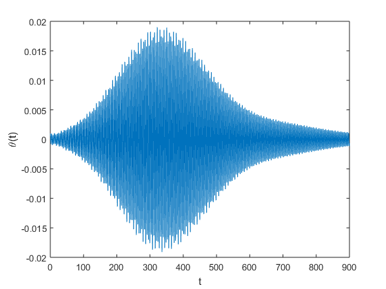
Successive doublings of the damping coefficient, produces the plots seen below, where throughout we have fixed the angular frequency \(\omega\) at 3. One can readily discern that increasing the damping coefficient the critical amplitude occurs at a later time. Possible design changes might include considering materials that naturally provide a higher damping coefficient, which would thus make the bridge less susceptible to torsion.
| d | \(\theta(t)\) | d | \(\theta(t)\) | d | \(\theta(t)\) |
| 2 | 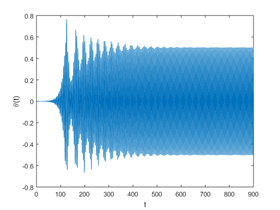 |
8 | 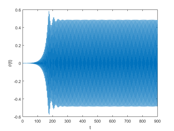 |
14 | 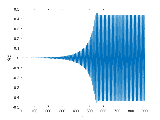 |
| 16 | 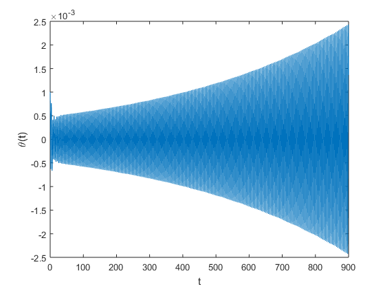 |
18 | 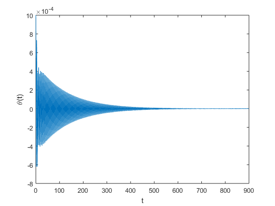 |
64 | 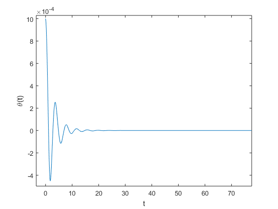 |