Project 1 |
|---|
Reality Check 1: Kinematics of the Stewart platformBy Julian Easley, Andrew Bender, and Mezel Simth |
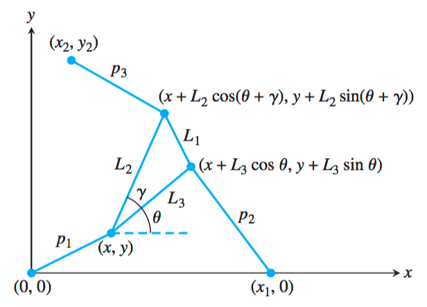
To further understand the nature of robotic arms, we will be investigating the kinetic nature of a 2D Stewart Platform. The platform investigated will consist of three hydraulic-assisted, variable-length struts connected to a triangular platform. In particular, we wish to find a way, given the current length of the struts, and the size of the platform, to determine what is the orientation and the location of the Stewart platform.
Utilizing the geometry of the above figure with arbitrary variables and constants, we arrive at the following equations:
\( \begin{align*} &A_2 = L_3\cos(\theta)-x_1\\ &B_2 = L_3\sin(\theta)\\ &A_3 = L_2\cos(\theta + \gamma) - x_2\\ &B_3 = L_2\sin(\theta + \gamma) - y_2\\ &N_1 = B_3 \left(p_2^2 - p_1^2 - A_2^2 - B_2^2 \right) - B_2\left(p_3^2 - p_1^2 - A_3^2 - B_3^2 \right)\\ &N_2 = -A_3 \left(p_2^2 - p_1^2 - A_2^2 - B_2^2 \right) - +A_2\left(p_3^2 - p_1^2 - A_3^2 - B_3^2 \right)\\ &D = 2\left(A_2B_3 - B_2A_3 \right)\\ \end{align*}\)
Given these equations, we arrive at a function of only one variable \(\theta\): \[f(\theta)=N_1^2 + N_2^2 - p_1^2D^2\]
Finding the roots of \(f(\theta)\) will provide us possible orientations the platform could take. Additionally, we have that: \[x=g(\theta)=\frac{N_1}{D}\] \[y=h(\theta)=\frac{N_2}{D}\] Therefore, we can determine x and y, along with the other two coordinates explicitly described in the above graph of \(f\), to ultimately determine the location and orientation of the platform.
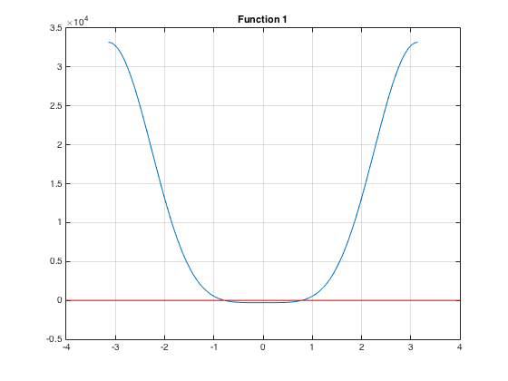
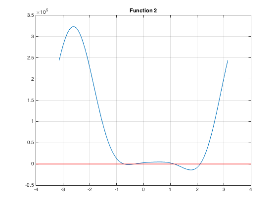
To get started, we tested plotting \(f(\theta)\) using the example values.
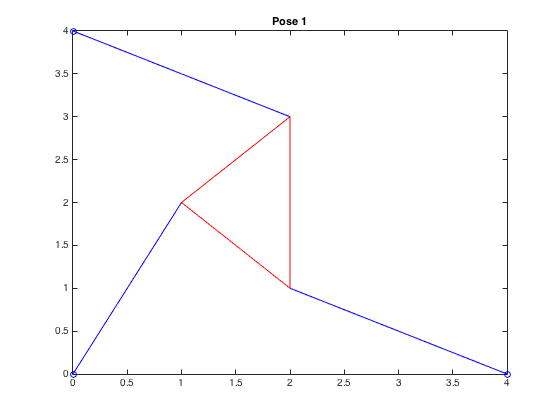
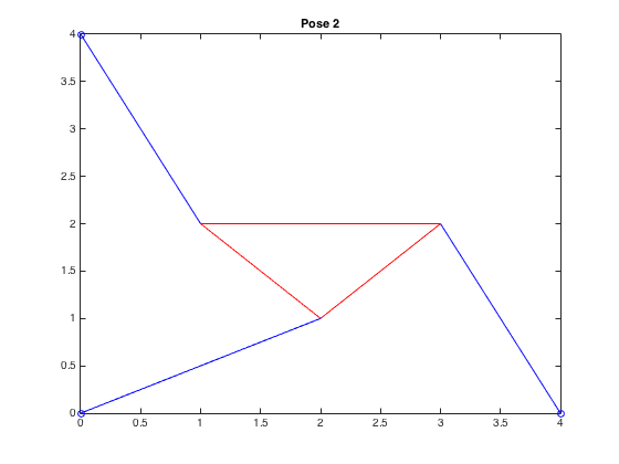
We proceded to plot the two possible poses given this \(f(\theta)\).
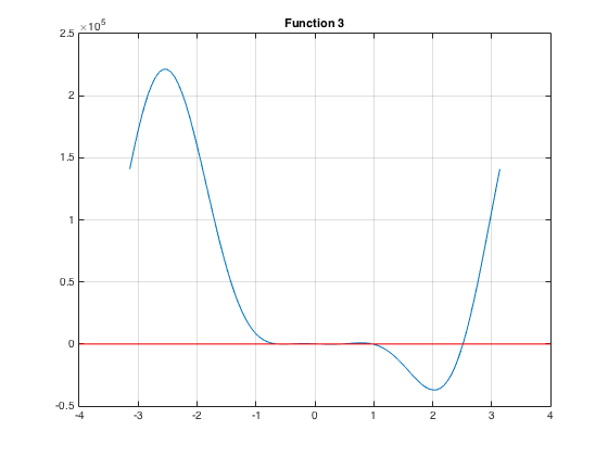
Changing the example to the specified ones we reploted the function.
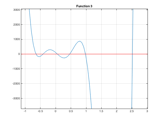
This image shows the roots more clearly:
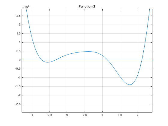
From the graph, we realized there exists four possible poses. In order to find the roots we use the bisection method.
| \( \boldsymbol{(x,y,\theta)} \) | Poses |
|---|---|
| \((-1.378,4.806,-0.721)\) | 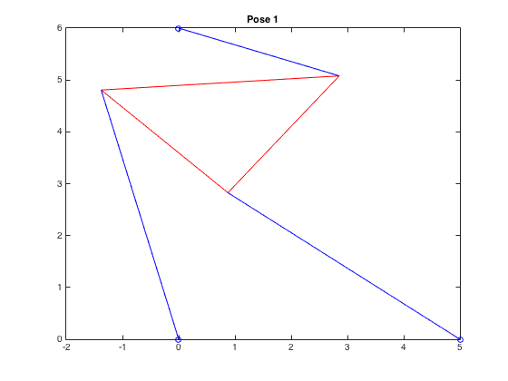 |
| \((-0.913,4.917,-0.330)\) | 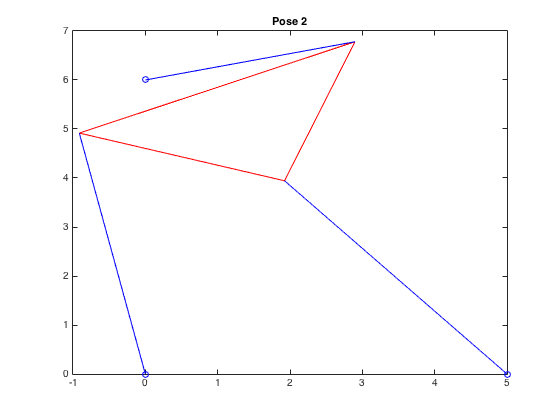 |
| \((4.483,2.220,1.143)\) | 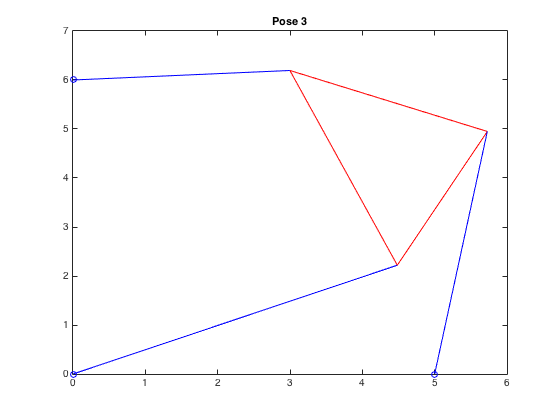 |
| \((4.572,2.025,2.116)\) | 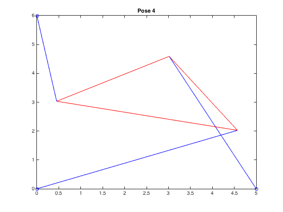 |
Here we investigate the effects of adjusting the \(p_2\) strut's length on the platform's location and orientation. We made \(p_2 = 7.01\). The same methods were used as before.
This image shows the roots more clearly:
From the graph, we realized there exists six possible poses.
| \( \boldsymbol{(x,y,\theta)} \) | Poses |
|---|---|
| \((-4.388,2.397,-0.641)\) | 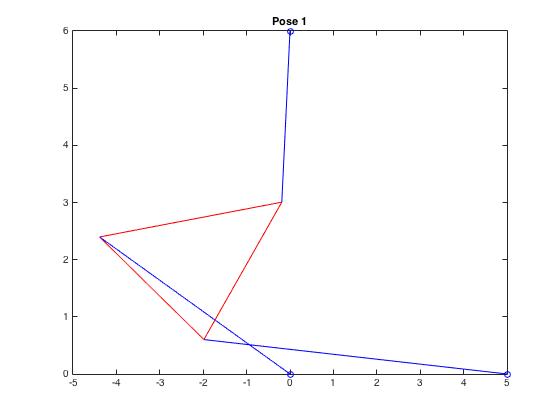 |
| \((-4.752,1.555,-0.410)\) | 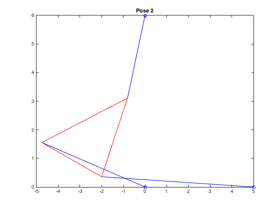 |
| \((-4.950,0.714,0.057)\) | 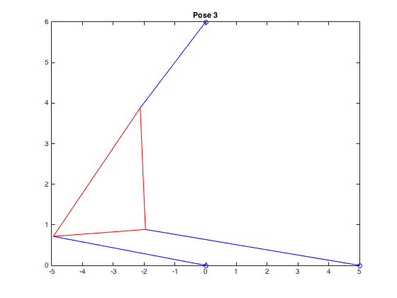 |
| \((-0.825,4.932,.462)\) | 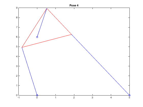 |
| \((2.287,4.446,.977)\) | 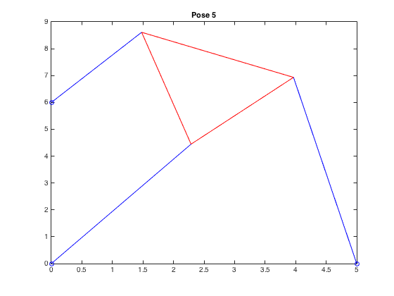 |
| \((3.207,3.836,2.515)\) | 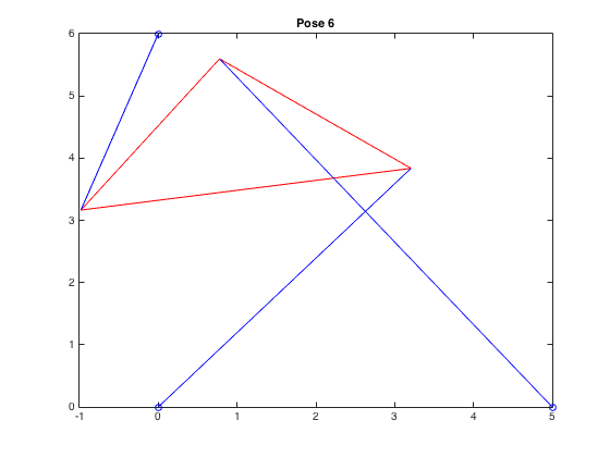 |
We change \(p_2\) again like the 3rd function but now \(p_2 = 9\).
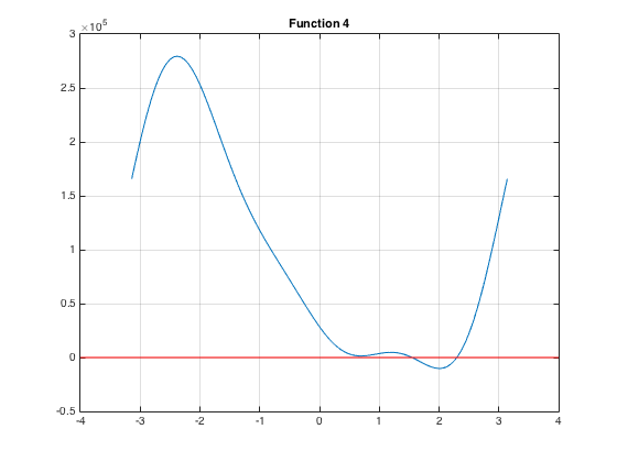
This image shows the roots more clearly:
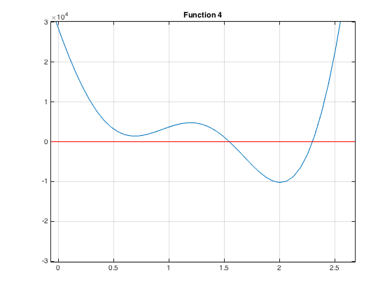
From the graph, we realized there exists two possible poses.
| \( \boldsymbol{(x,y,\theta)} \) | Poses |
|---|---|
| \((0.709,4.950,1.548)\) | 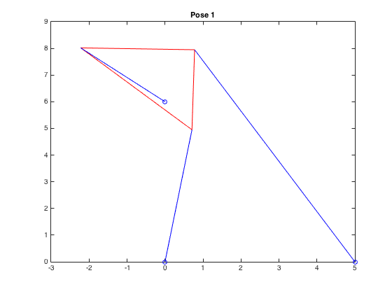 |
| \((1.392,4.803,2.299)\) | 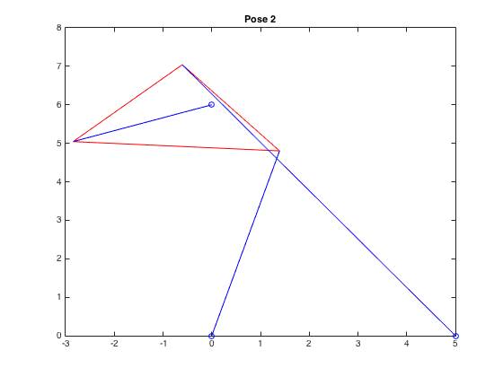 |