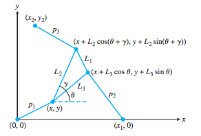
This project explores a 2-dimensional version of the Stewart Platform, a problem that arises frequently in robotics, and in which the position of a platform is controlled by variable strut length. In this project, we were tasked with finding the position of a triangular platform (the variables x,y, and θ) given the lengths of the struts (\(p_1,p_2,p_3\)) and their fixed endpoints. Click the link for more of the project details.
Our code for f(\(\theta\)) can be viewed here. We graphed f(θ) for the known values L1=2, L2 = L3 = \(\sqrt{2}\), \(\gamma\)=\(\frac{\pi}{2}\), p1 = p2 = p3 = \(\sqrt{5}\) on the interval \([-\pi,\pi]\). The two roots at \(\frac{-\pi}{4}\) and \(\frac{\pi}{4}\) are visible on the graph below.
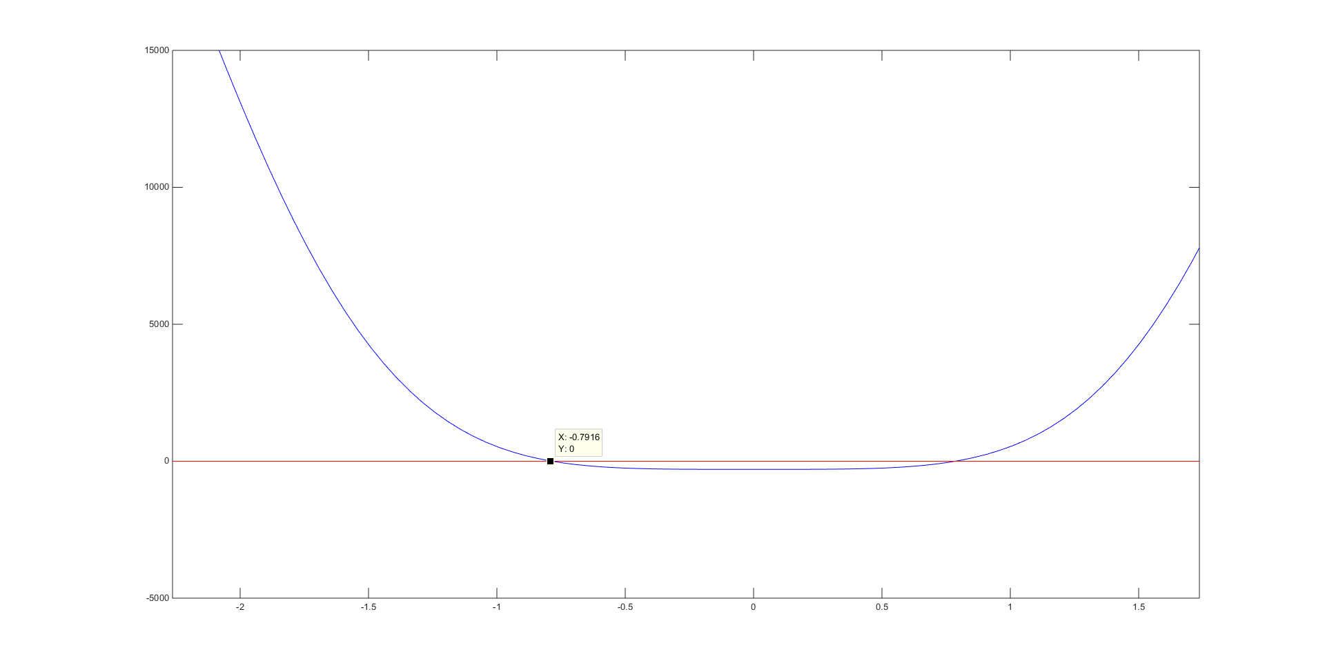
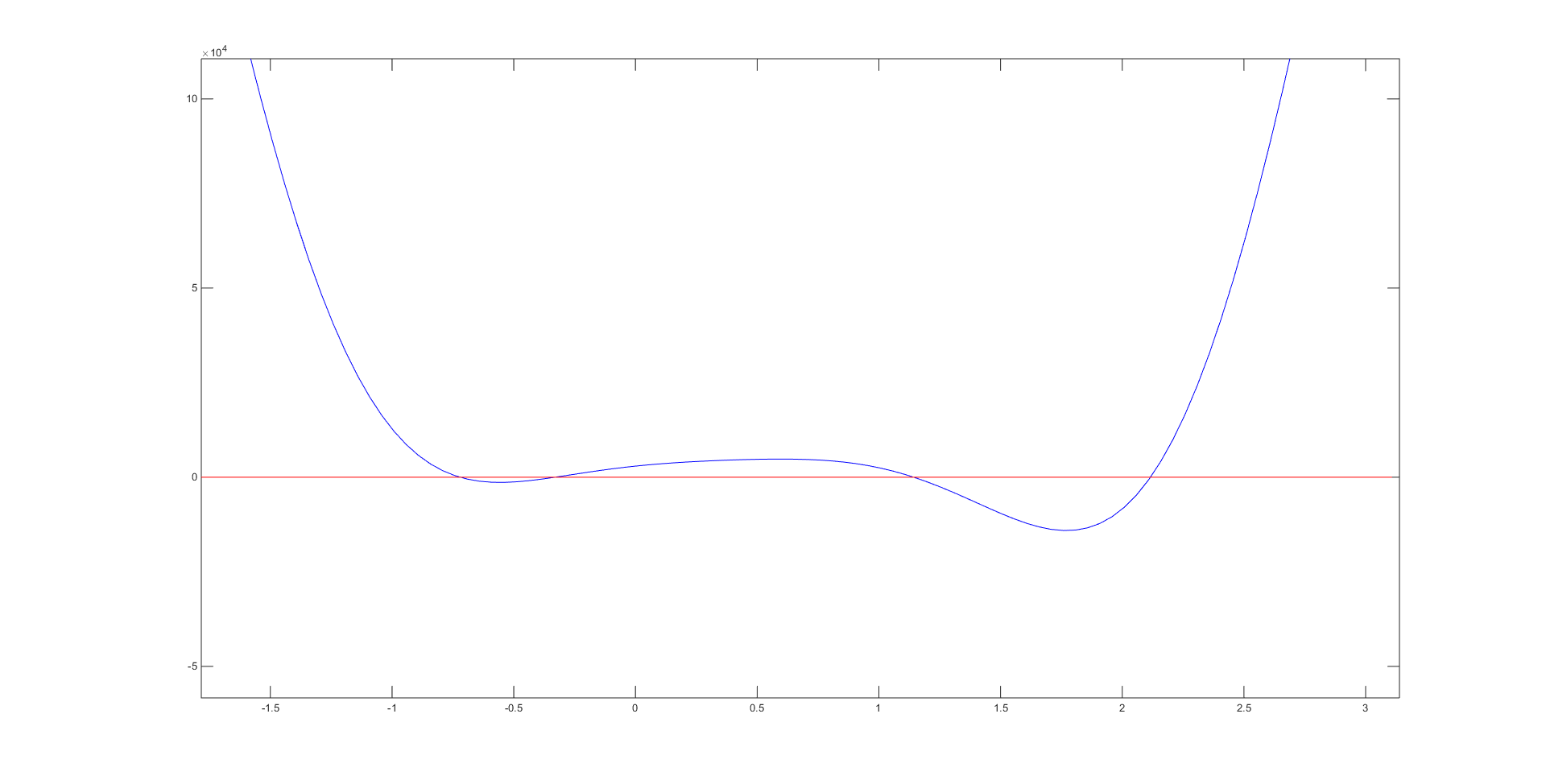
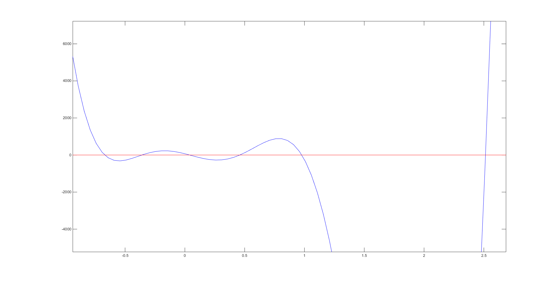
In part 4, we were actually tasked with developing a root finding method to solve for \(f(\theta) = 0\) with the parameters \(x_1 = 5, (x_2, y_2) = (0,6), L_1 = L_3 = 3, L_2 = 3\sqrt{2}, \gamma = \frac{\pi}{4}, p_1 = p_2 = 5, p_3 = 3\). Our group chose the bisection method, as with sufficient initial guesses, convergence to the roots is always guaranteed. By generating the plot of \(f(\theta)\) below, we could easily see there were 4 roots and obtain valid initial guesses for each root.
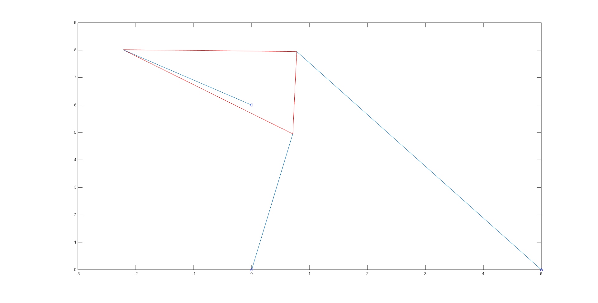
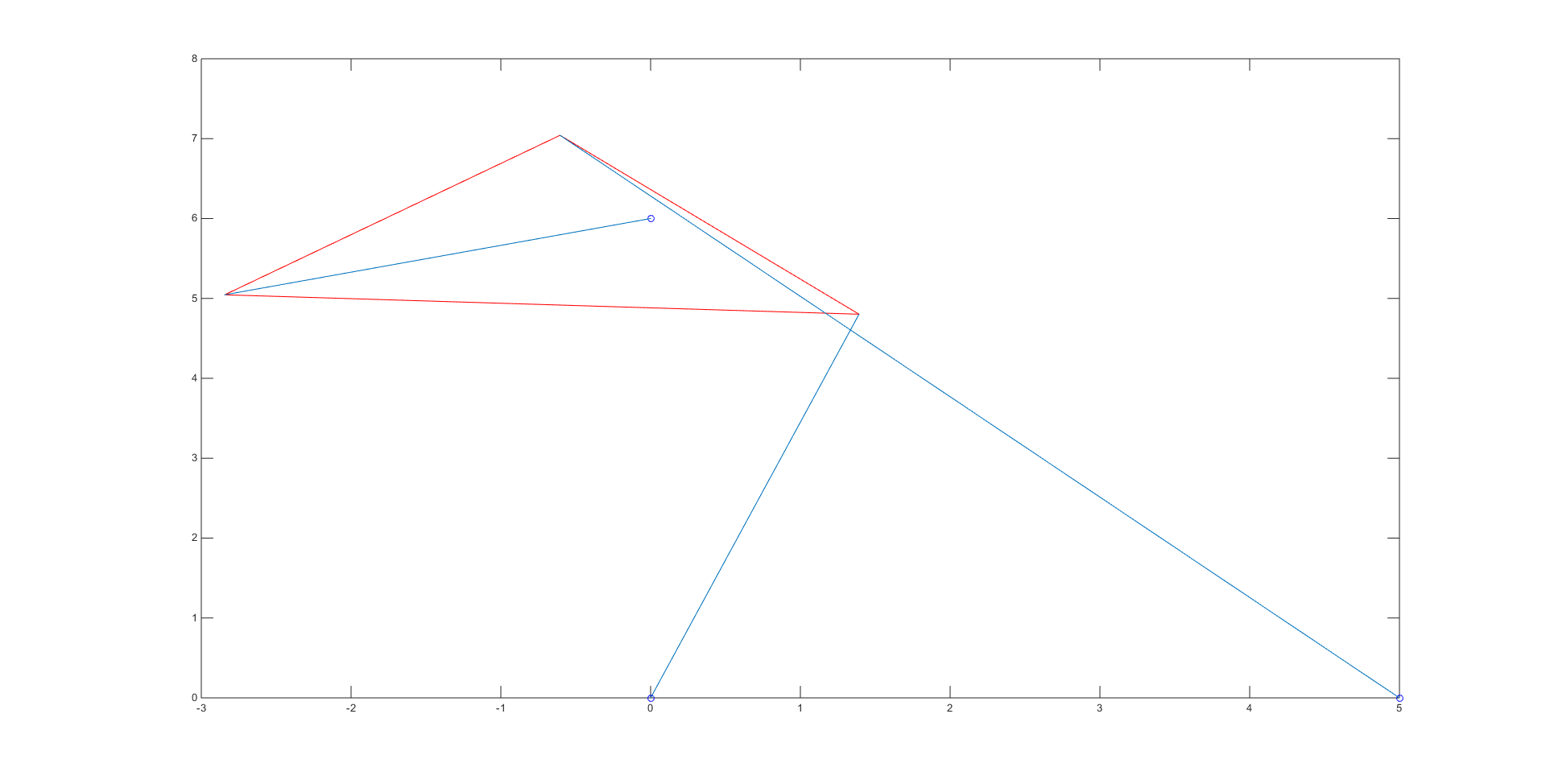
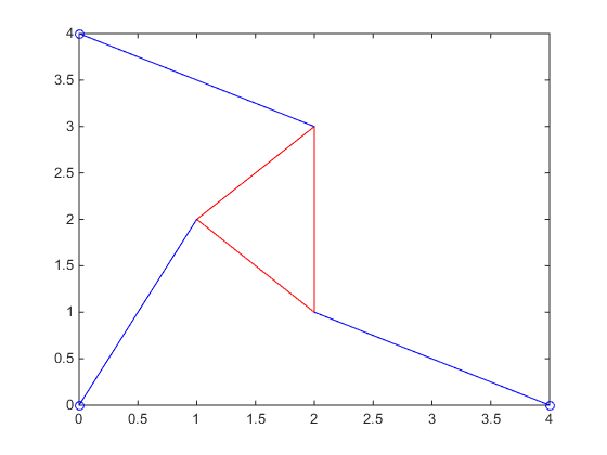
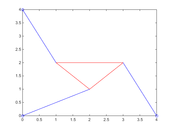
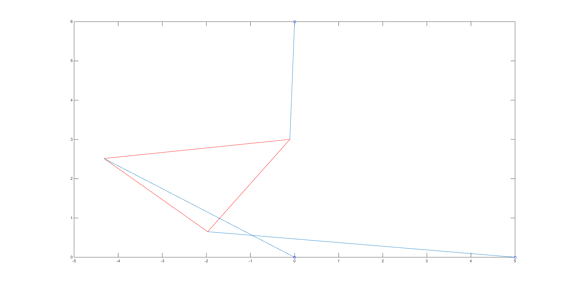
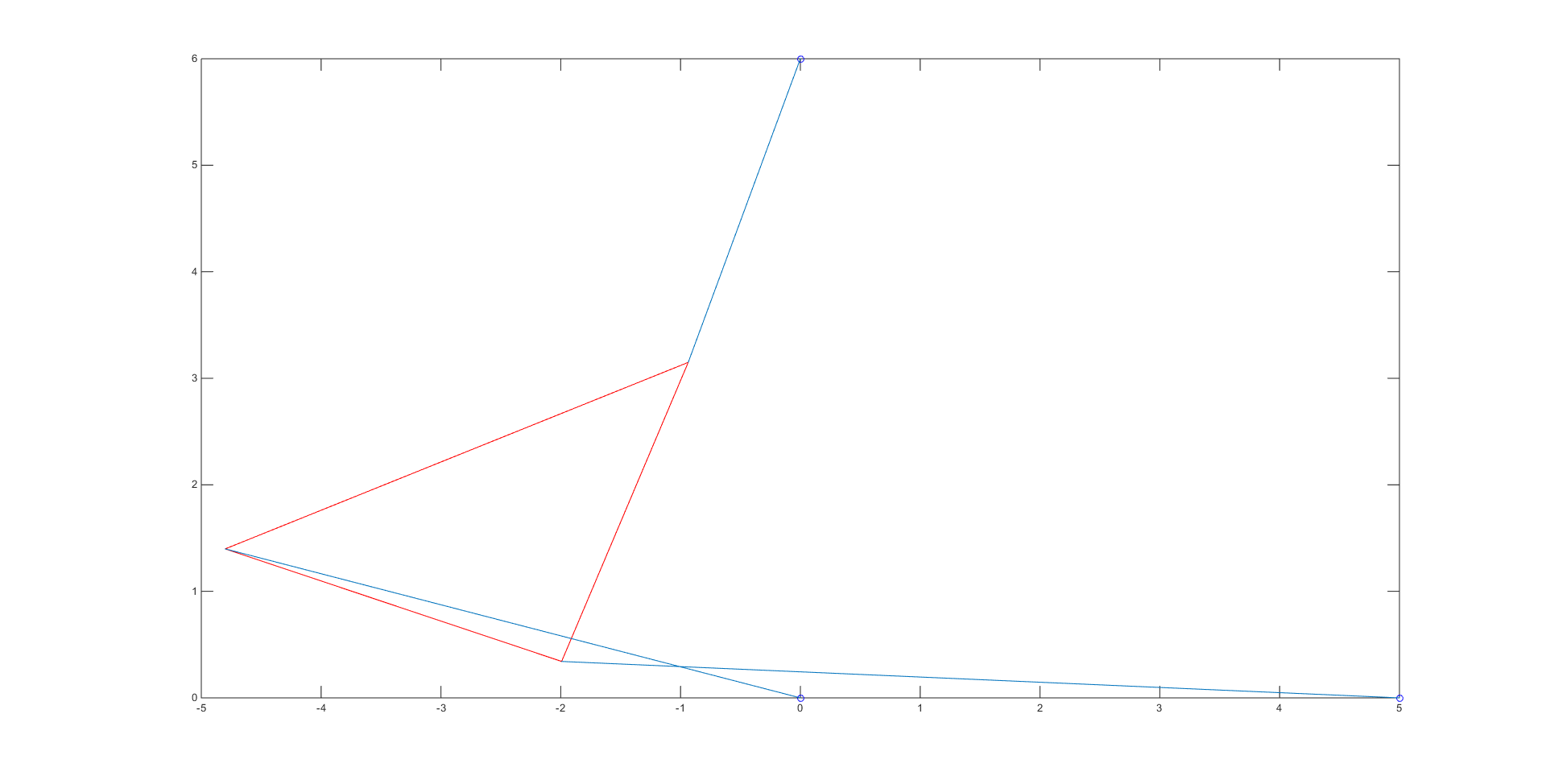
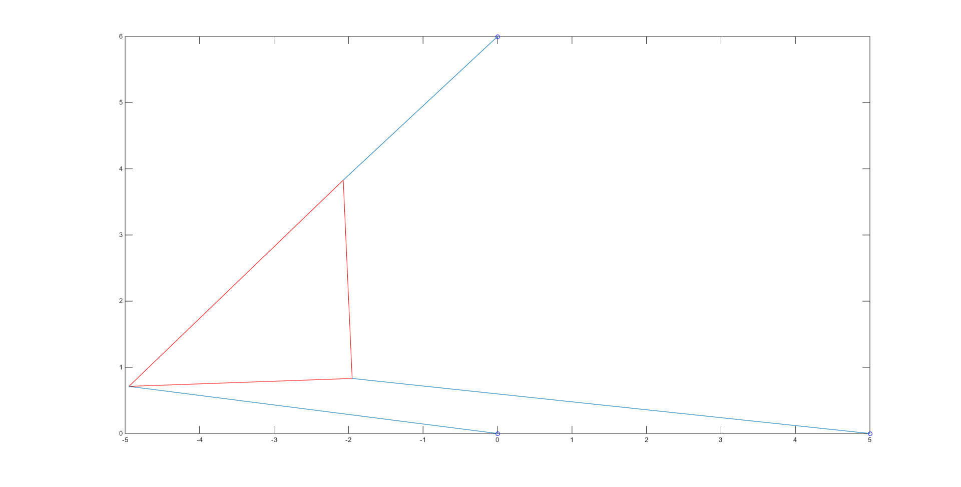
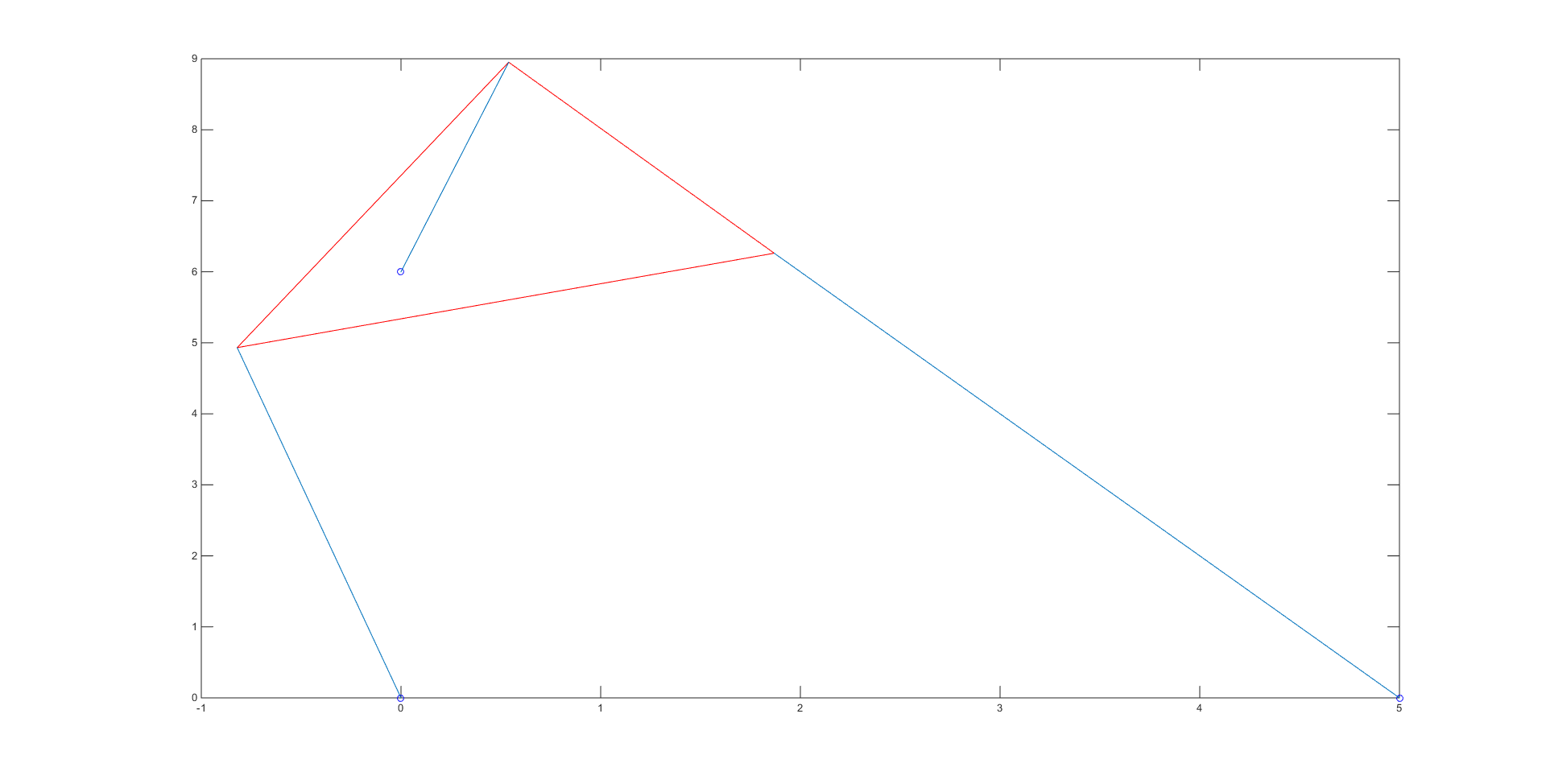
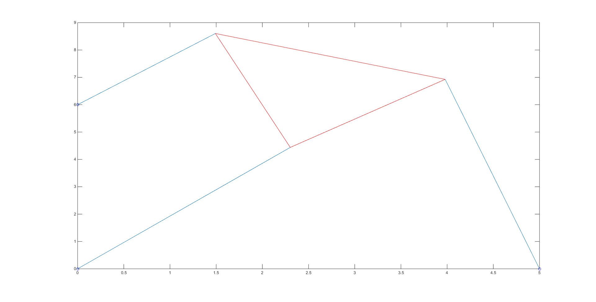
Our bisection method code, which contains the initial guesses used for each root, can be viewed here. The bisection code spit out the numerical values of the roots \(\theta\), which we then put into coordinates to obtain the vertices of our platform and plot the different poses. There were a total of 4 roots: -0.7208, -0.3310, 1.1437, and 2.1159, giving us the 4 poses shown below:
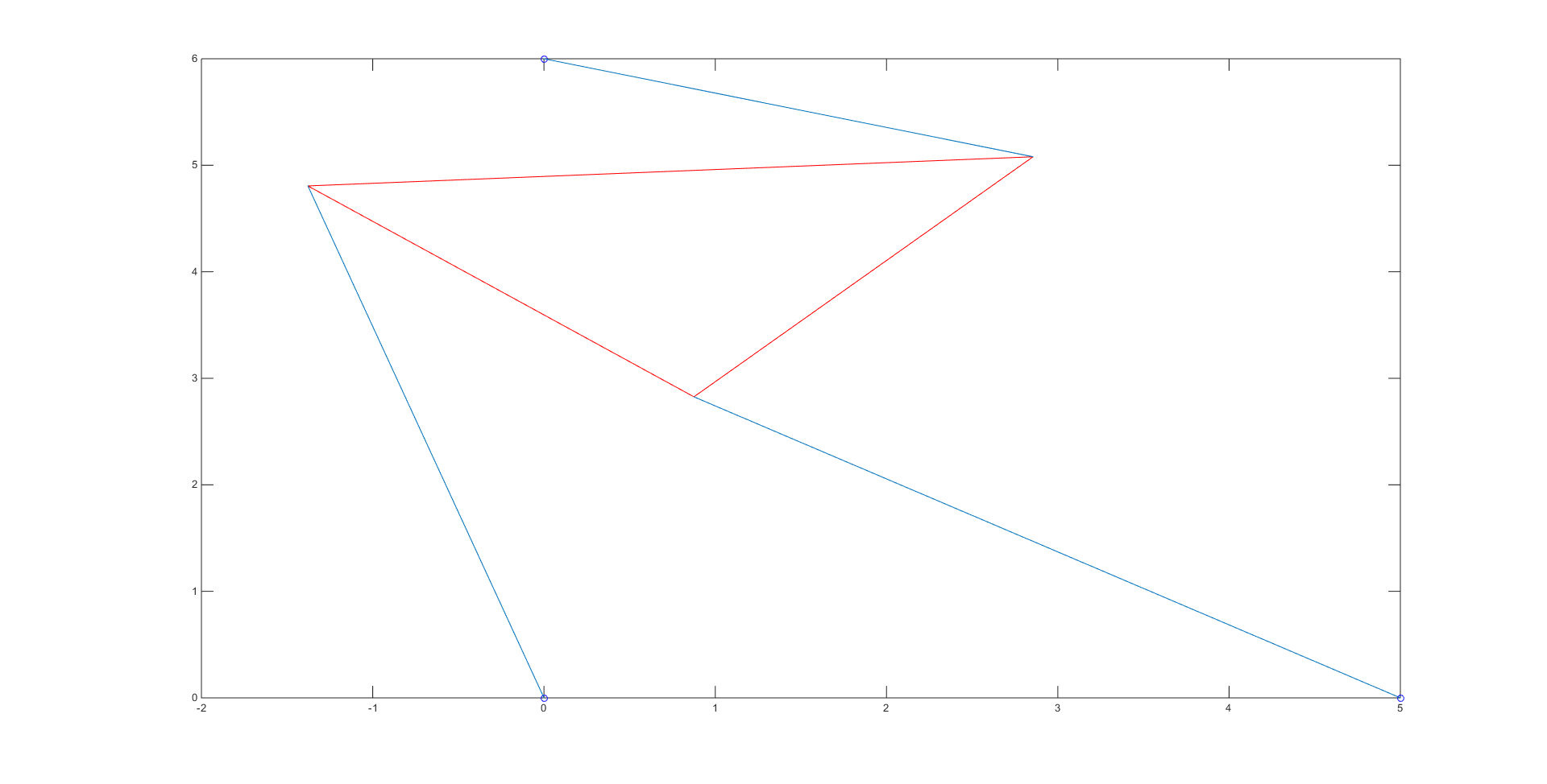
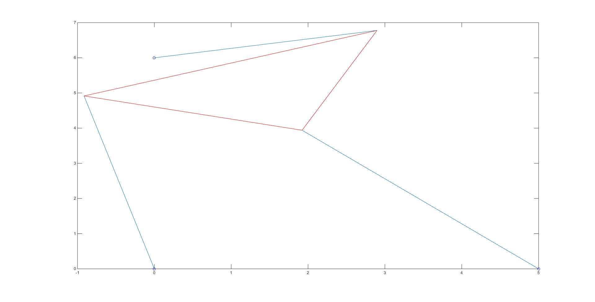
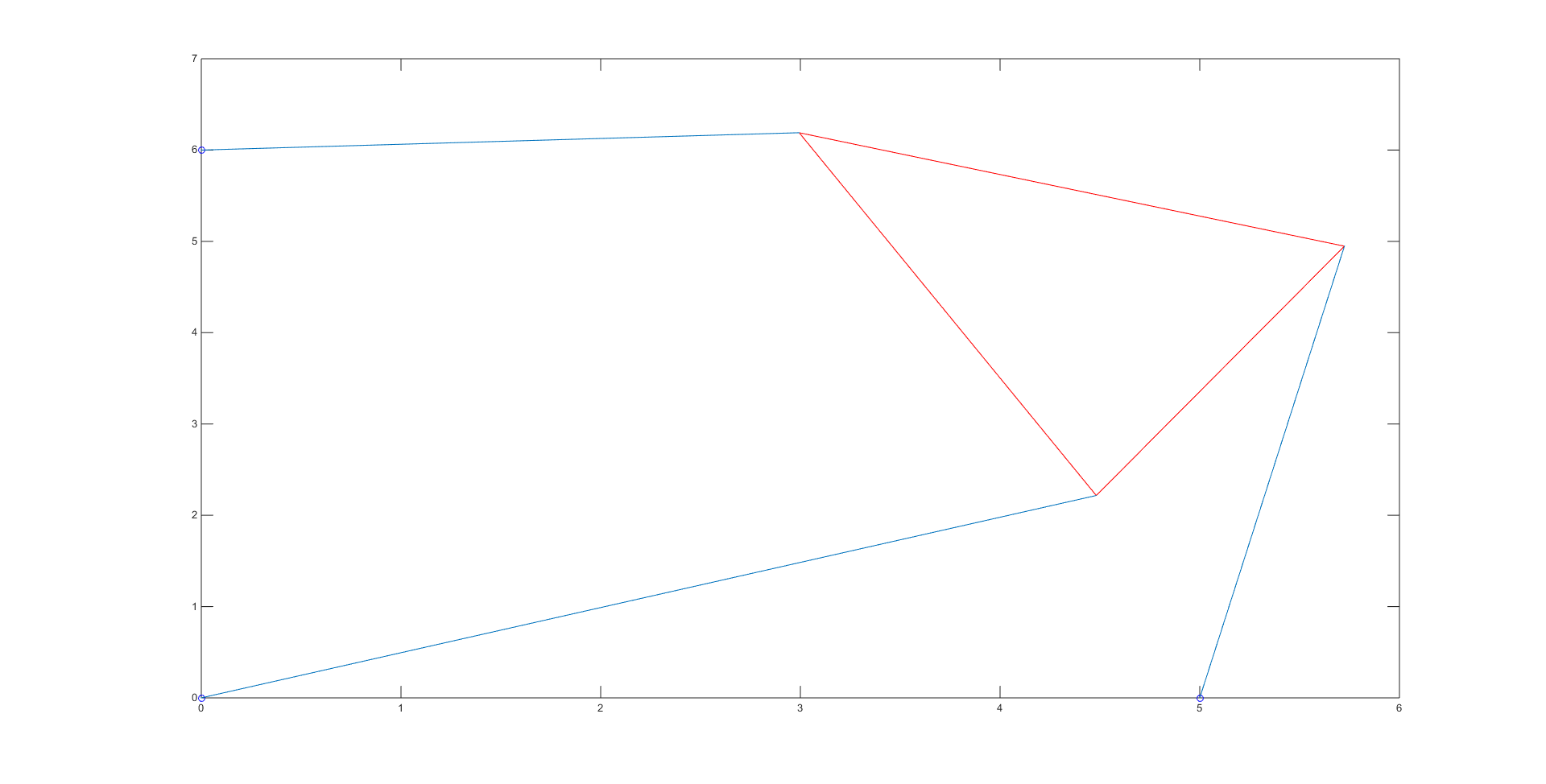
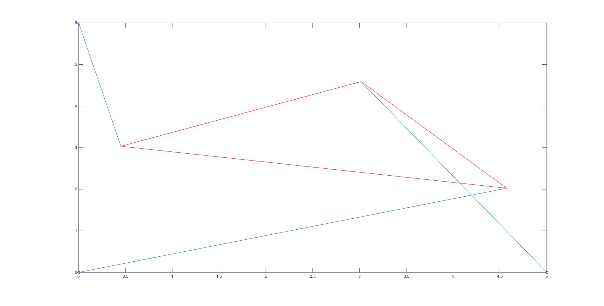
In order to check that each of these poses had the correct length, we simply checked the distance between the given strut endpoints and the calculated vertices for the 3 blue lines in each of the poses using the simple distance formula.
The only difference between parts 5 and 4 was the \(p_2\) value, which we changed to 7.001 and re-solved for a total of 6 different roots and so 6 different poses. The graph of \(f\theta)\) for this new \(p_2\) value is shown below:
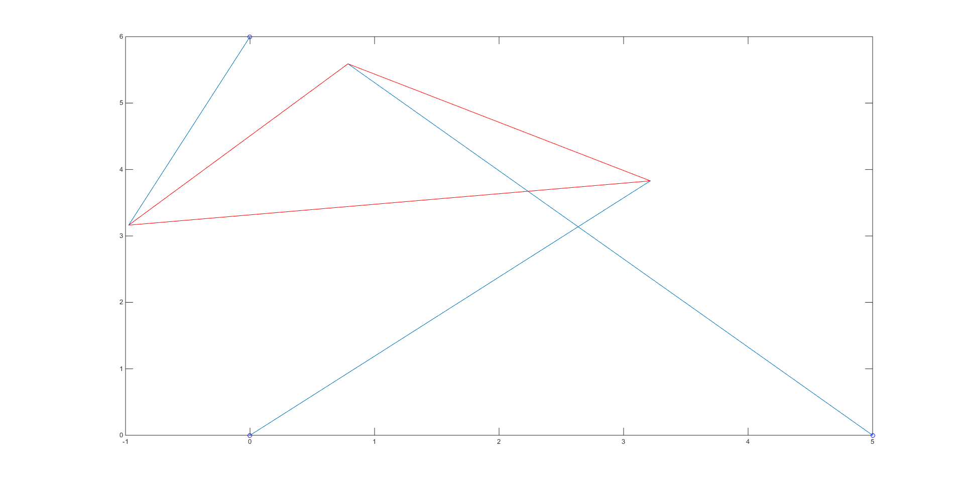
The 6 roots were: -0.6704, -0.3600, 0.0399, 0.4592, 0.9776, and 2.5139. Their plots can be seen below
Lastly, we were tasked with finding a \(p_2\) value that produced only 2 roots. After graphing a few different \(f(\theta)\), we found that \(p_2\) = 9 produced the following plot
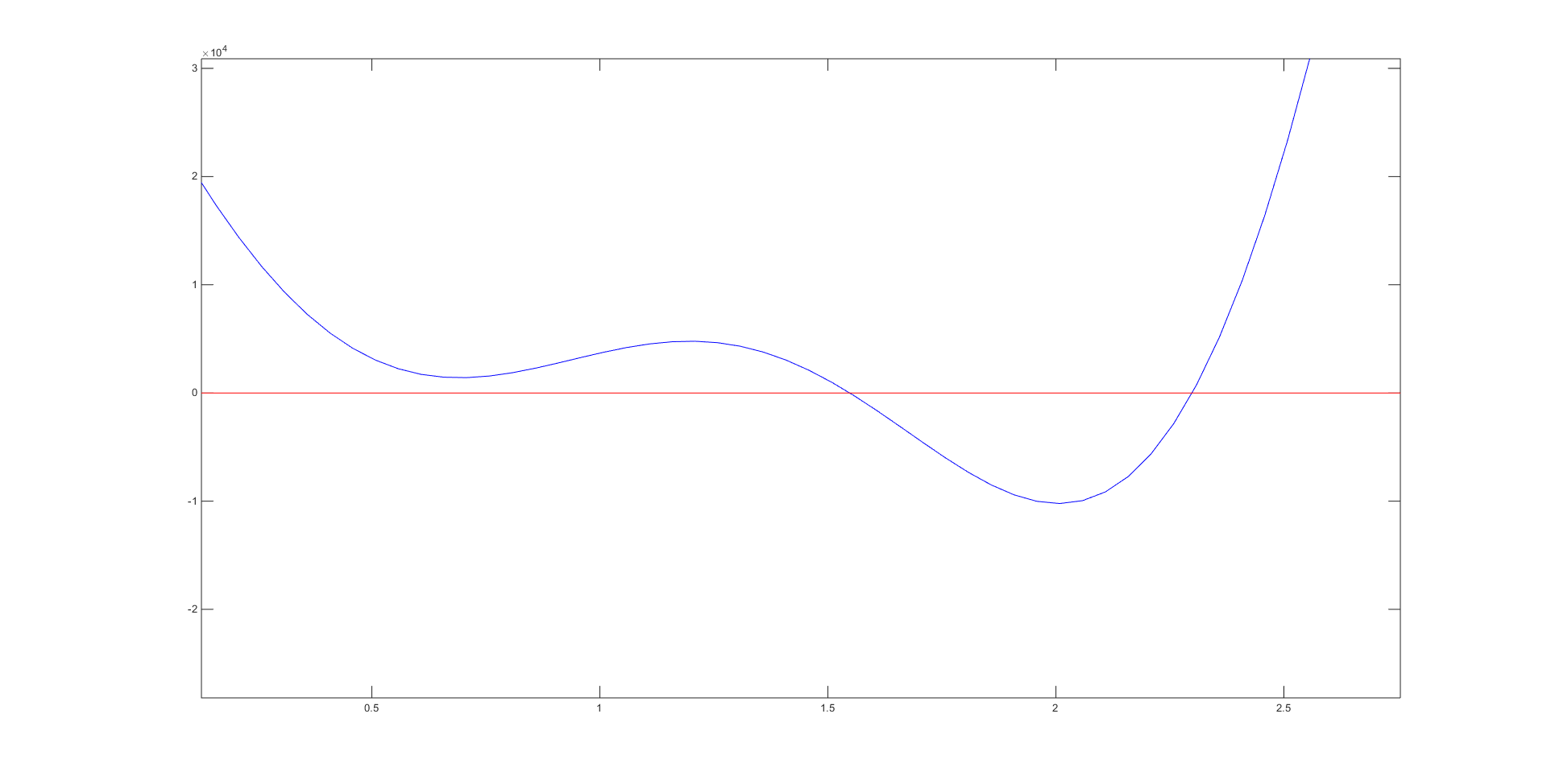
Plugging this new value in, we obtained the roots 1.5479 and 2.2989 with their associated poses