For this project we used the 2-dimensional discrete cosine transform to compress images, meaning that we essentially represent the images using less data, and re-expand out this information using the inverse transform to recreate the images. Some information is lost each time, but as we will see, with certain quantization techniques this loss can be imperceptible.
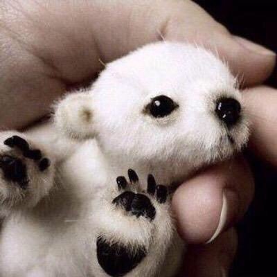
For the first part, we were asked to compress a greyscale image in 8x8 blocks, and put these blocks back into an image. The original image I chose was 400x400 (keeping it simple with square dimensions divisible by 8):
Using the MATLAB commands
x = imread('baby_animal.jpg');
x=double(x);
r=x(:,:,1);g=x(:,:,2);b=x(:,:,3);
xgray=0.2126*r+0.7152*g+0.0722*b;
it was possible to turn this into a greyscale photo, shown below

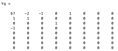
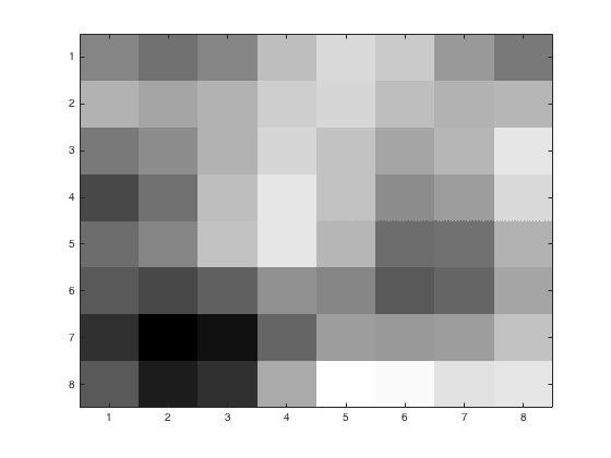
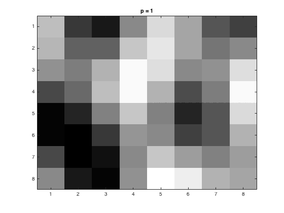
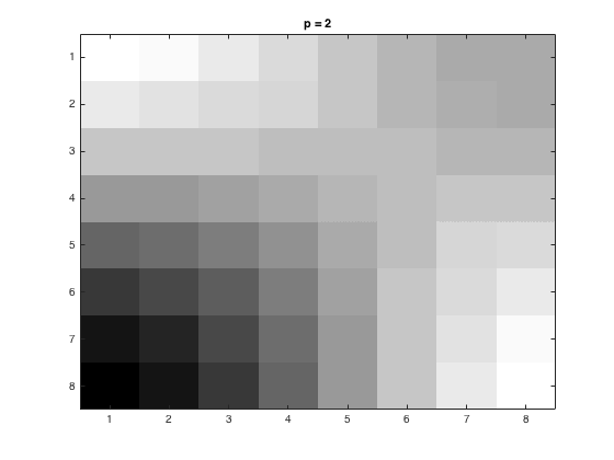
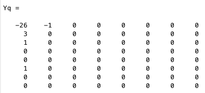
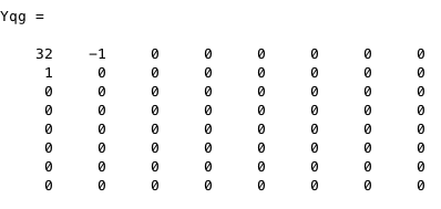
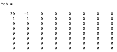
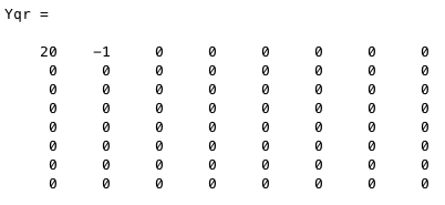
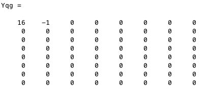
The first task was to divide this up into 8x8 pixels with varying \(p\) values. Before the data was re-expanded, the following matrices stored the information for the 1:8x1:8 square for \(p = 1, 2, 4\) respectively.
 |
 |
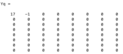 |
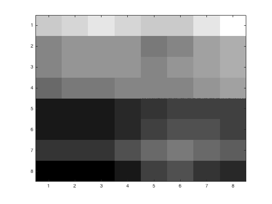
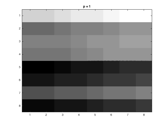
Below is the 1:8x1:8 square, and the values of \(p = 1, 2, 4\) respectively. These figures were generated using the code here.
 |  |  | 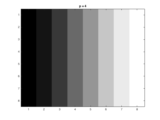 |
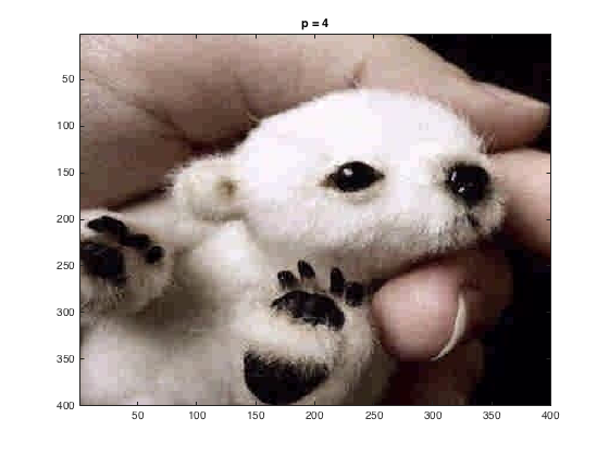
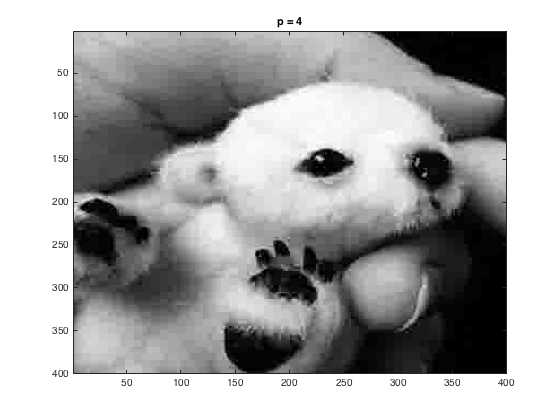
Next, we were to do this for every 8x8 square on the 400x400 picture, and put these squares together into one image. For this, I made use of 2 nested for loops, one to keep track of columns, the other rows in our final matrix. The code for this part is provided here. Upon closer inspection, you can see more quality loss the higher \(p\) gets.
 |
 |
 |
Next, still in greyscale, we were to quantize the data using the JPEG suggested matrix, given here
\(Q = p\left( \begin{array}{cccccccc} 16& 11& 10& 16& 24& 40& 51& 61\\ 12& 12& 14& 19& 26& 58& 60& 55\\ 14& 13& 16& 24& 40& 57& 69& 56\\ 14& 17& 22& 29& 51& 87& 80& 62\\ 18& 22& 37& 56& 68& 109& 103& 77\\ 24& 35& 55& 64& 81& 104& 113& 92\\ 49& 64& 78& 87& 103& 121& 120& 101\\ 72& 92& 95& 98& 112& 100& 103& 99 \end{array} \right) \)With \( p = 1\), the data for the square 81:88x81:88 was stored in the matrix and can be seen against the original image below.
 |
 |
|
 |
That code is given here.
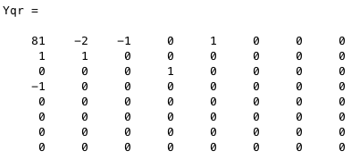
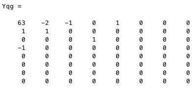
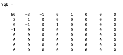
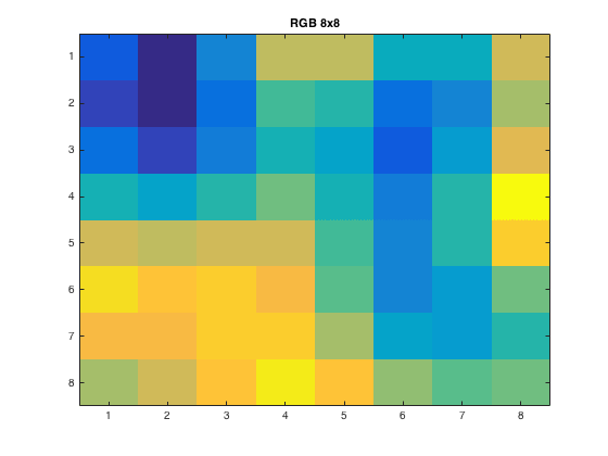
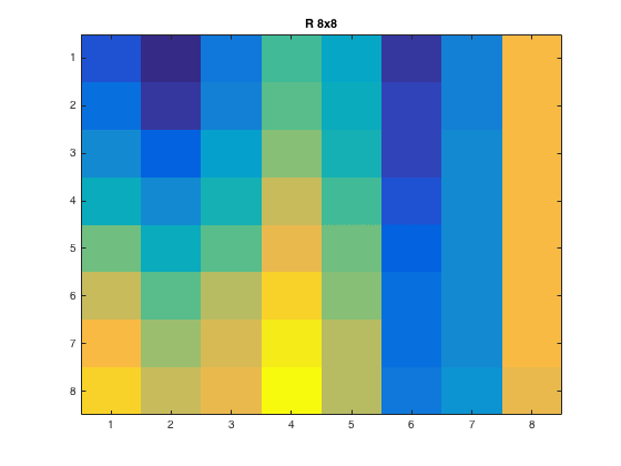
Next we were to repeat the steps in part 3, but this time in RGB. We were to quantize the different colors separately, and then put them all together in the end to show the final picture. The code for this part is given here.
 |
 |
 |
 |
 |
 |
 |
 |
 |
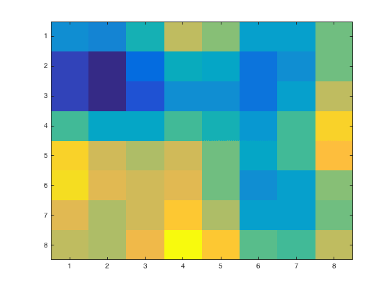
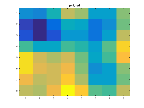
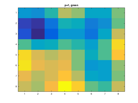
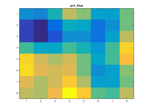
For the 1:8x1:8 pixel and \(p=1\), this is what the output showed
 |
 |
 |
 |
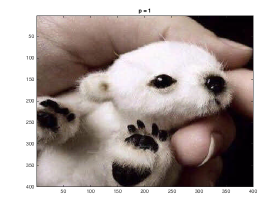
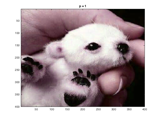
Putting them all together, we have the following images for \(p = 1, 2, 4\) respectively. The first image shows the orginal color image.
|
 |
 |
 |
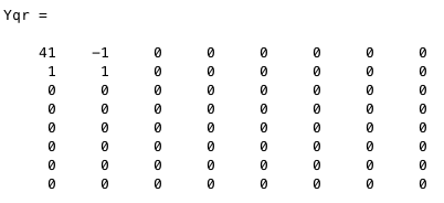
Finally, we were to transform the RGB coordinates to the luminance (Y) and color difference coordinates (U,V) given by
The code for this part is given here. For the \(p = 1\) case we have the following images shown against the original
 |
 |
 |
 |
Finally, I put the images together to obtain for \(p = 1, 2, 4\)