Black and White Image Compression

Kathleen McLane

Linear Quantization

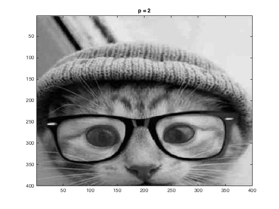
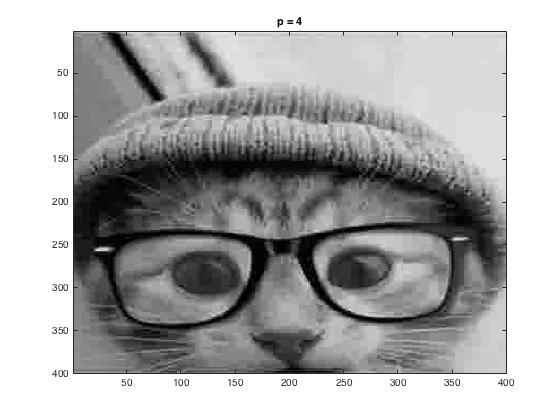
The first two questions for this project involved performing image compression on a black and white image. The image that was used for this project is of a cat wearing glasses. Using MATLAB's commands, I was then able to change it to a black and white image, this can be seen here.

The first question involved selecting an 8x8 pixel block, applying the 2D-DCT to it, quantizing it for linear quantization for when p=1, 2, and 4, reconstructing the block using the inverses 2D-DCT, and then repeating this for the entire image. The code for this work can be seen here. The 8x8 plot that was selected can be seen below:

Next the \(Y_Q\) was found, and the print outs for p=1,2, and 4 can be seen below. The matrix for p=1, \(Y_Q\)= \begin{bmatrix} 14 & -1 & 0 & 0 & 0 & 0 & 0 & 0\\ 0 & 0 & -3 & 0 & 0 & 0 & 0 & 0\\ 0 & 0 & 0 & 0 & 0 & 0 & 0 & 0\\ 0 & 0 & 0 & 0 & 0 & 0 & 0 & 0\\ 0 & 0 & 0 & 0 & 0 & 0 & 0 & 0\\ 0 & 0 & 0 & 0 & 0 & 0 & 0 & 0\\ 0 & 0 & 0 & 0 & 0 & 0 & 0 & 0\\ 0 & 0 & 0 & 0 & 0 & 0 & 0 & 0\\ \end{bmatrix} The matrix for p=2, \(Y_Q\) = \begin{bmatrix} 7 & -1 & 0 & 0 & 0 & 0 & 0 & 0\\ 0 & 0 & 0 & 0 & 0 & 0 & 0 & 0\\ 0 & 0 & 0 & 0 & 0 & 0 & 0 & 0\\ 0 & 0 & 0 & 0 & 0 & 0 & 0 & 0\\ 0 & 0 & 0 & 0 & 0 & 0 & 0 & 0\\ 0 & 0 & 0 & 0 & 0 & 0 & 0 & 0\\ 0 & 0 & 0 & 0 & 0 & 0 & 0 & 0\\ 0 & 0 & 0 & 0 & 0 & 0 & 0 & 0\\ \end{bmatrix}

The matrix for p=4, \(Y_Q\) = \begin{bmatrix} 3 & 0 & 0 & 0 & 0 & 0 & 0 & 0\\ 0 & 0 & 0 & 0 & 0 & 0 & 0 & 0\\ 0 & 0 & 0 & 0 & 0 & 0 & 0 & 0\\ 0 & 0 & 0 & 0 & 0 & 0 & 0 & 0\\ 0 & 0 & 0 & 0 & 0 & 0 & 0 & 0\\ 0 & 0 & 0 & 0 & 0 & 0 & 0 & 0\\ 0 & 0 & 0 & 0 & 0 & 0 & 0 & 0\\ 0 & 0 & 0 & 0 & 0 & 0 & 0 & 0\\ \end{bmatrix}

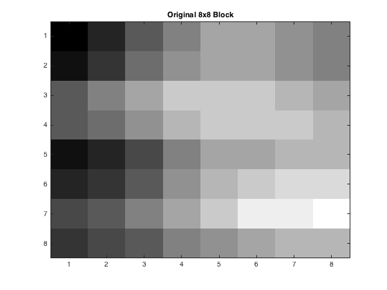
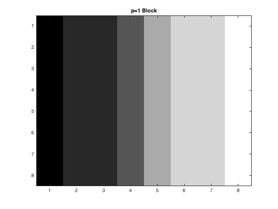
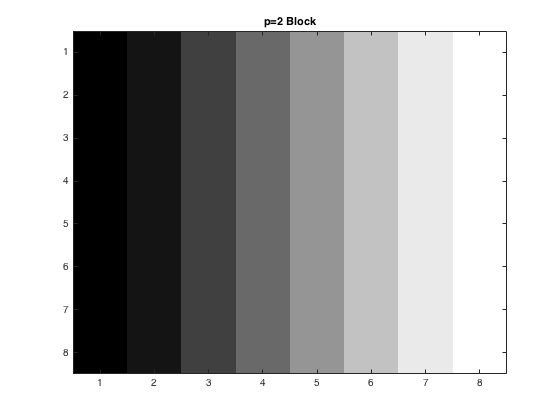
After the \(Y_Q\) plots were found, the inverse was taken for each case, and the completed pictures were reconstructed. First though, the new 8x8 blocks were printed out. These can be seen below. As the quality of the picture was not the best, it can be seen as p gets larger, the detail used quickly diminishes, where by the time p=4 comes around, all the detail is lost.

Once this was completed for an individual 8x8 block, the picture was then put back together. This produced a compressed picture for when p=1,2,and 4. The new three pictures can be seen below, where by the time it gets to p=4 the whole picture looks very grainy. The code for this can be seen here.

JPEG Quantization

The next part of the problem involved completing the above steps, but instead of using linear quantization, the JPEG matrix was used instead. This matrix looks like:

\begin{bmatrix} 16&11&10&16&24&40&51&61\\ 12&12&14&19&26&58&60&55\\ 14&13&16&24&40&57&69&56\\ 14&17&22&29&51&87&80&62\\ 18&22&37&56&68&109&103&77\\ 24&35&55&64&81&104&113&92\\ 49&64&78&87&103&121&120&101\\ 72&92&95&98&112&100&103&99\\ \end{bmatrix}

Using this matrix instead of the linear quantization one, and a value of p=1 for the loss parameter, new images were produced. The new \(Y_Q\) looks like: The matrix for p=1, \(Y_Q\) = \begin{bmatrix} 3 & -1 & 0 & 0 & 0 & 0 & 0 & 0\\ 3 & 0 & 0 & 0 & 0 & 0 & 0 & 0\\ 2 & 0 & 0 & 0 & 0 & 0 & 0 & 0\\ 1 & 0 & 0 & 0 & 0 & 0 & 0 & 0\\ 0 & 0 & 0 & 0 & 0 & 0 & 0 & 0\\ 0 & 0 & 0 & 0 & 0 & 0 & 0 & 0\\ 0 & 0 & 0 & 0 & 0 & 0 & 0 & 0\\ 0 & 0 & 0 & 0 & 0 & 0 & 0 & 0\\ \end{bmatrix}

Continuing with the inverse 2D-DCT, and then putting the image back together provides a compressed image. The difference between the original and the compression is almost not noticeable, which is what is to be expected.