Math 447 Project 4: Heat Distribution on a Cooling Fin
In this project, the Heat Distribution on a Cooling Fin was modeled. The equation used to model the Heat Equation is given below:
Where K represents the thermal conductivity of an aluminum fin, 1.68 W/cm degree Celsius, H is the transfer coefficient = 0.005 degrees Celsius,
and delta represents the width of the fin in mm.
This equation is formally known as an Elliptic Partial Differential Equation. In our model, power is input along the left side of the fin, on an interval of [0,L], where L represents the length of the fin in cm. It is worth noting the length of the heat input does not have to be for the entire length of the fin. For example one could input the power (in Watts), over only half of the fin size, for example. This situation was investigated in Problem 2 of the project.
The equation representing the power, entering the fin on it's left side, is given by Fourier's Law:
Where L and K are the same as they were as stated previously, and P represents power in watts.
In order to approximate the PDE, the finite difference method was implemented in Matlab. This method divides the domain of the problem in a M x N grid, and uses the Taylor Series approximation of the second derivative in x and y to approximate a solution to the PDE.
1. In the first problem, a fin of dimensions 2 x 2 cm, with 1 mm thickness was modeled with a power input of 5 Watts. The grid used to model the equation was 40 x 40. With an ambient room temperature of 20 degrees Celsius, the maximum temperature of the fin was shown to be 165 degrees Celsius. This is very hot!
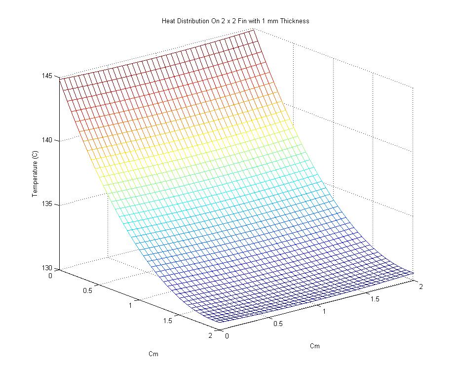
Code Here
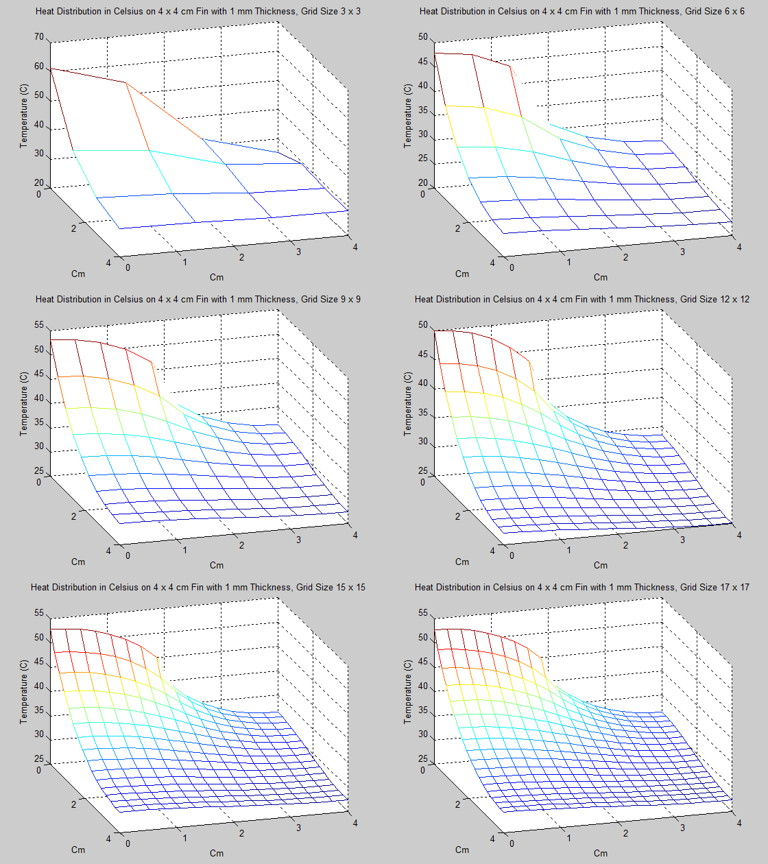
2. In the next problem, the dimensions of the fin were changed to 4 x 4 cm, with thinkness 1 mm. This time however, power was input of the interval of [0,2], which represents exactly half of the length of the left side. As one might expect, the maximum temperature of the fin was significantly cooler than it was in Problem 1. Also of interest in this problem was seeing the effect that increasing the grid size had on the solution. This is shown in the animation below, starting with a grid size of 3 x 3 and ending with a grid size of 17 x 17. Unfortunately, the method used for creating gifs in Matlab would not accept grid sizes greater than 17 x 17. Grid sizes starting at 20 x 20 increasing by increments of 5 are shown below the animation.
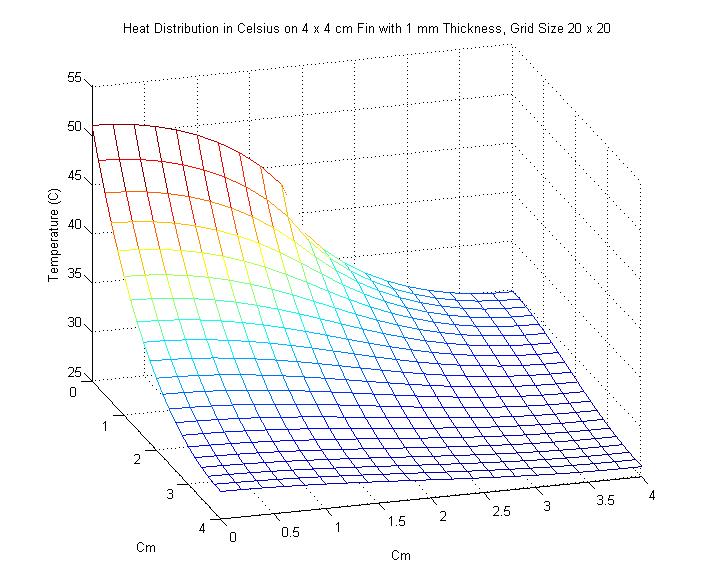
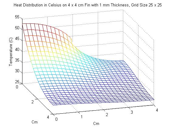
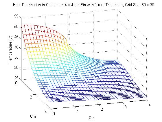

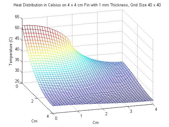
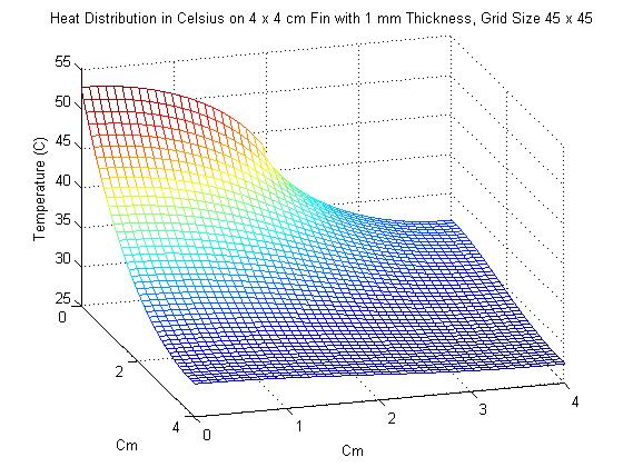
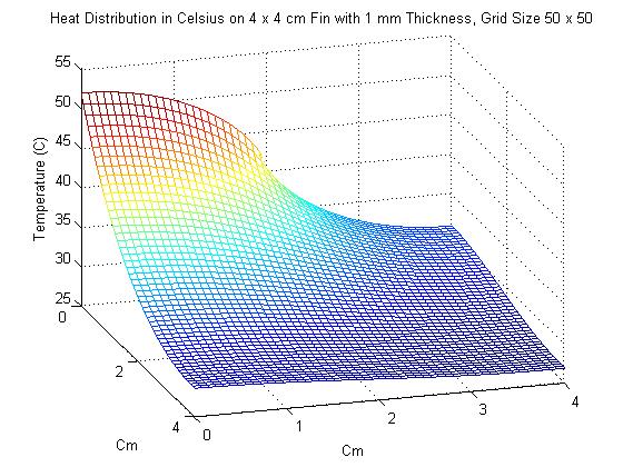
As one can see, changing the grid size has a definite effect on the approximation of the Heat Distriubution.
Code Here
The next portion of the project is located on my partner Wonjun Lee's Website: 3,4 and 5
The last portion of the project is located on my partner Aaron McPhee's Website: 6 and 7
References
Sauer, T. Numerical Analysis 2nd Ed. Pearson