Home
Project Details 1 2 3

Math 447 Project 2: GPS, Conditioning, and Nonlinear Least Squares

Chris Mazzullo and James Trichilo

This project used numerical methods to solve for an individual's position on the Earth, given a set of initial conditions. In the case of GPS, the initial conditions were the positions of the satellites in orbit (in km), and the differences in transmission time between the satellite and the individual receiving the signal. Once these problems were solved, further examinations were in order. What would happen if the transmission time was manipulated by a factor of $10^{-8}$ seconds? Accordingly, all possible manipulations were calculated to determine the maximum error of such discrepancies. This process also revealed an important issue with GPS — should the satellites be in a very close range of each other, a high amount of error in location will occur. Lastly, the Gauss-Newton method was used to determine if adding more satellites, eleven to be specific, would add any degree of precision.

1. The following equations describe the GPS Problem:

$(x-A_1)^2 + (y-B_1)^2 + (z-C_1)^2 = [c(t_1-d)]^2$

$(x-A_2)^2 + (y-B_2)^2 + (z-C_2)^2 = [c(t_2-d)]^2$

$(x-A_3)^2 + (y-B_3)^2 + (z-C_3)^2 = [c(t_3-d)]^2$

$(x-A_4)^2 + (y-B_4)^2 + (z-C_4)^2 = [c(t_4-d)]^2$

In fact, this is the equation for a sphere, centered at A, B, and C, where Ai, Bi, and Ci, are the respective locations of the satellite. In order to solve for x, y, z, and d Newton's Multivariate Method was used. This method is completely analogous to Newton's Method in one variable, however, with multiple variables, one has to invoke the Jacobian, a matrix of partial derivatives, and then iterate. In this problem, the Jacobian is:

Newton's Multivariate Method was then implemented and very quickly converged to the roots of the equations:

$(x,y,z,d) = (-41.77271, -16.78919, 6370.0596, -.003201566).$

Code Here

2. In the second problem, the first problem was solved again in a different manner. If one examines the equations in Figure 1, one will notice that by factoring the square of variable in parenthesis6 and subtracting Row 1 from each equation, they can obtain a system of linear equations. Specifically, by using algebra and factoring out the variables, they can put the equation into a new form:

$x\vec u_x + y\vec u_y + z\vec y_z + d\vec u_d + \vec w = 0$

From here, a very interesting attribute of determinants can be used to solve for x, y, and z. Determinants are linear, meaning one can pull out constants or variables associated with a column or row of the Matrix. For example, the following procedure was used to generate an equation for x:

$0 = det[\vec u_y|\vec u_z|x\vec u_x + y\vec u_y + z\vec u_z + d\vec u_d + \vec w]$

From the equation above, one can pull the x, y, z, and d out of the matrix's by the linearity of determinants. Further examination of the second and third matrix's will show that they have repeated columns. The second matrix has the uy repeated, and the third matrix has uz repeated. Any matrix with a repeated column will have a determinant of zero, thus the y and z variable will be multiplied be zero, leaving only variables x and d. From here, an equation for x, in terms of d, can be determined. This process can be repeated with a shuffling of the columns, to generate equations for y and z in terms of d.

With equations for x, y, and z in terms of d now determined, one can then plug these equations into any row of the equations in Figure 1, and they will now have a quadratic equation in d. This process is very messy on paper, and can be made immensely easier using Matlab's symbolic representation of variables. By declaring d a symbolic variable, one can then generate their equations for x, y, and z in terms of d, then directly plug them into any of the rows in Figure 1.

% Solve for x in terms of D

XColumn = [Uy Uz Ux];

DColumn = [Uy Uz D];

wColumn = [Uy Uz w];

% Determinant of X, d, and w

xDeterminant=det(XColumn);

Ddet = det(DColumn);

wDet = det(wColumn);

% Declare symbolic variable

syms d

% Equation for x

x = (-d*Ddet - wDet) / xDeterminant;

After repeating for x, y, and z, one can directly plug them into the equation and solve it:

% Plug x, y, and z into the equation and solve

fun = ((x)-A1)^2 + ((y)-B1)^2 + ((z)-C1)^2 - (c*(t1-d))^2;

% Roots of the equation

roots=double(solve(fun));

r1=roots(1);r2=roots(2);

% Plug both roots into x y and z

x1 = double(subs(x,d,r1))

y1 = double(subs(y,d,r1))

z1 = double(subs(z,d,r1))

x2 = double(subs(x,d,r2))

y2 = double(subs(y,d,r2))

z2 = double(subs(z,d,r2))

% See the back error of the calculations

check = (x2-A1)^2 + (y2-B1)^2 + (z2-C1)^2 - (c*(t1-r2))^2

The following values were determined using this implementation:

x2 =

-41.772709570837364

y2 =

-16.789194106526853

z2 =

6.370059559223343e+03

r2 =

-0.003201565829594

check =

The values for x, y, z, and d match those calculated by Newton's Multivariate Method in problem 1.

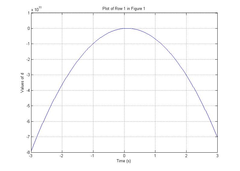
This plot above is given by the equation:

$(83788.807142489154347391948011069*d + 14038.195822626503377827117747065)^2 + + ( 623.67719529477219334465494718772*d + 7558.7859377036797065250420180836 )^2 + ( 10.749177881495164086481966417906*d - 15641.738295370235739880023862907)^2 -( 299792.45799999998416751623153687*d - 21207.318478919998880010098218918)^2$

with roots at:

$r 1 = 0.185173047095946$

$r 2 = - 0.003201565829594$

Code Here

3. Now that an understanding of the problem and means of solving it were developed, the next step was to manipulate the values for t, where t is the difference between the times the signal was transmitted and received. In this problem, spherical coordinates were used for the locations of the satellites:

$A_i = pcos(\phi)cos(\theta)$

$B_i = pcos(\phi)sin(\theta)$

$C_i = psin(\phi)$

Where p = 26570 km, phi is between or equal 0 and pi/2, and theta is between or equal 0 and 2 pi.

The transmission difference would be moved up or down by $10^{-8}$ seconds. This may seem like an incredibly small amount of time, however, when multiplied by the speed of light, this amounts to about 3 meters. In other words, a very slight change in transmission time could cause various degrees of errant locations by the GPS. Just how great might these changes be?

In order the quantify this, the following formula was used:

$EMF = \frac{||\delta x,\delta y, \delta z||\infty}{c||\delta t_1,...,\delta t_m||\infty}$

Where c denotes the speed of light, delta denotes change in, and infinity symbol denotes the infinity norm

In order to determine the greatest quantity, a method was developed by Chris that systematically went through every combination, be it satellite 2 and 3 delayed, satellite 1 delayed and 3 advanced, etc...to determine the greatest value of the EMF. After going through all 81 possibilities, each of which being iterated by Newton's Multivariate Method 10 times, the following values were computed:

Maximum Position Error = 19.95 meters

EMF = 6.650

Code Part I Here

Code Part II Here

4. The process detailed in part 3, was repeated again with satellites grouped with both phi and theta within 5% of each other. In this implementation, Chris, in a very similar manner to the methodical approach of the previous problem, performed 10 iterations with random values of phi and theta within 5% of each other. Due to the use of randomly generated numbers, this function does not yield the same output every time. After many iterations, the highest number we generated was:

maxerror = 6.691893380212397e+03

In other words, a maximum position error of 6,691 kilometers (6,961,000 meters), with an EMF of 2.230631126737466e+06. Not good!

Code Part I Here

Code Part II Here

5. For the last problem, we were to add an arbitrary number of satellites between five and twelve, but not eight. It was decided that we would examine what would happen if eleven satellites were used to locate a persons location, and determine if adding additional satellites would add any degree of precision. In order to solve this, the Gauss-Newton Method was implemented.

The Gauss-Newton Method is very similar to the Multivariate Newton's Method. Once again, a Jacobian of partial derivatives was calculated, this time for eleven satellites, and used to iterate towards a solution. However, with eleven satellites, one now has eleven equations in four unknowns. An efficient way to deal with this is through the lens of least squares. The equation for the Gauss-Newton Method is given by:

$D\vec F(x_0)^T * D\vec F(x_0) * \vec v = -D\vec F(x_0)^T * \vec F(x_0)$

$\vec x_i = x_0 + \vec v$

Where DF represents the Jacobian, x0 is initial guess, and xi represents the next guess to be iterated

It is worth noting that just like with the normal equations, the Gauss-Newton Method is a projection onto a vector.

Going back to ideas presented in part three, we bring back the notions of the EMF and the Maximum Position Error. Again, the difference in transmission time is manipulated by a factor of $10^{-8}$ , and the effects of various manipulations are determined. The following results were seen:

If there were no manipulations in the eleven transmission times, the accuracy was spectacularly good. The Maximum Position Error is on the order of millionths of inches with an EMF of .003.
The satellites were sensitive to transmission manipulations. Iterations performed with all eleven satellites being manipulated caused various degrees of position error.
A wide range of initial guesses would converge (guesses between (0,0,0,0) to (5000,5000,5000,5000) were tested).

All possible combinations were not tested in this instance. From the iterations that were performed, however, the following results are reported with eleven satellites:

Maximum Position Error = 5.855 meters

EMF = 1.951749599660009

Code Here

Summary

This project was fascinating and very rewarding. Based on our results, we conclude that adding additional satellites is of benefit in adding degrees of precision to a location. Our results with eleven satellites showed a marked improvement over our results with four satellites. On the other hand, we have also shown that using closely bunched satellites can have disastrous effects. Our maximum error was on the order of thousands of kilometers! If one was in Washington D.C., a closely bunched GPS system could place one in London, Rio De Janeiro, or even the North Pole. Not only was learning about GPS great, but we also gained a familiarity with more sophisticated numerical methods...home run!

References

Sauer, T. Numerical Analysis 2nd Ed. Pearson

First image courtesy of http://images.iop.org/objects/phw/news/16/4/10/gps.jpg

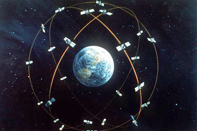
Second image courtesy of http://rammb.cira.colostate.edu/dev/hillger/GPS-constellation.jpg