Haar and Daubechies Wavelets via Gabriel Peyré
Part VII: 2-D Daubechies Wavelets
In this section, with the help of Mr. Peyrę, I extend another dimension to the Daubechies Wavelet. This enables me to use a greyscale picture. Again, the FWT (Forward Wavelet Transform), will be implemented. We use the Daubechies "D4" Wavelet was use 2 vanishing moments. This means a polynomial of degree 1 can be accurately represented. I attempted to explain what vanishing moments are at the end of my 1-D Daubechies section. In regards to the FWT, it is nice because it can be viewed in terms of recurisive filtering. From the filtering perspective, it is simply repeated discrete time convolutions of the low and high pass filters. The same filters used in the 1-D section are used in this section as well.
The frequency response of these filters is plotted below.
As one might expect, the added dimensions makes the FWT a little more complicated. At each stage, a filtering and downsampling is performed in the horizontal direction, and then in the vertical direction. (1)
The superscript H indicates that this is in the horizontal direction. Thus, we are operating on the columns of the picture matrix. Next, we operate in the vertical direction, on the rows of the matrix.
Mr. Peryę shows this on his site as well.
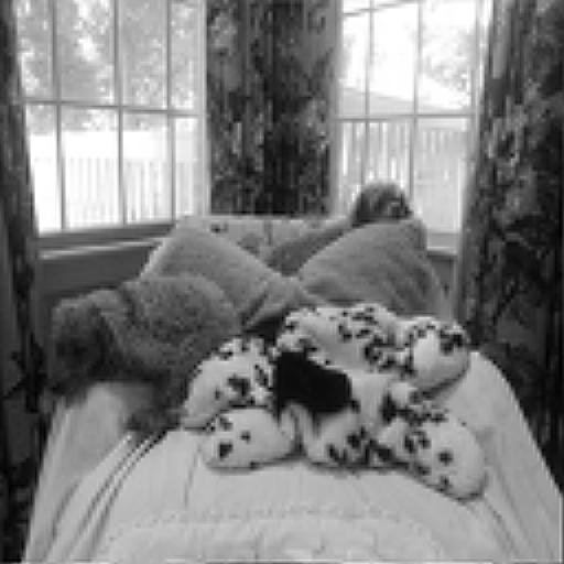
This is the image I will be performing the 2-D FWT with Daubechies Wavelets on.
Here is the first step of the FWT with the Daubechies Wavelets. The first step was performined in the vertical direction. The top half of the transformed plot shows the low pass coefficients after downsampling, and the bottom half shows the high pass coefficients after downsampling.
This is the result of the transform after iteration in the horizontal direction.
Now, a the full FWT is implemeneted. Because multi-resolution is awesome, we examine the some of the middle stages of the FWT.
This is implemented by performing the FWT is both the vertical and horizontal dimension. We can now observe the picture of the dogs at different scales in different dimensions. Perhaps not terribly amazing in its own right, but nevertheless, still amazing that we are able to do that. Below, all the Wavelet Coefficients are plotted.
Inverse 2-D FWT
As j increases, the image gets better. This is because at each stage of reconstruction, more Wavelet coefficients are being used to piece the signal back together. Here is the fully reconstructed image.
The error between the original and reconstructed image? 9.6625e-12! Amazing.
Filtering
As usual, Non-Linear Filtering is implemented as well. This process is very simple. One chooses a certain threshold of their liking, and then filters all coefficients below that threshold. A threshold of .2 is used in this instance, which filters out many Wavelet coefficients.
The Non-Linear filtering is quite a bit more effective than the Linear Filering.
Here is the linearly filtered image:
Here is the non-linearly filtered image:

The aren't perfect, and some would say not great either. It reminds me a lot of Skype video quality. I can't help but suspect that Skype uses a lot of compression in their video streaming. Mr. Peryę then implements a fascinating method were he uses different wavelets with more vanishing moments. He uses the DB2, DB4, and DB3 Wavelets in his implementation. Surprisingly enough, it turns out that the best approximation came from the Haar Wavelet! The Haar Wavelet is equivalent to the DB2 Wavelet. Mr. Peryę used the previously seen hibuscus, and in the case of that image, the DB6 filter was the best. The first image below is the Haar version, and the second one is the original. Keep in mind that all images in the iteration had the .2 Non-Linear filtering applied to them. This image is not perfect, but I think it is better than the previous two filtered images above.
Conclusion
Works Cited
(1) Peyrč, Gabriel. "2-D Daubechies Wavelets." 2-D Daubechies Wavelets. N.p., 2010. Web. 28 June 2014.
G. Peyré, The Numerical Tours of Signal Processing - Advanced Computational Signal and Image Processing, IEEE Computing in Science and Engineering, vol. 13(4), pp. 94-97, 2011.