Celestial Mechanics

Vincent Caetto, Jason Lasseigne, and Tim Reid

Introduction

Celestial mechanics is the study of the motion of large objects through space like planets and stars. Systems of linear differential equations are used to model the motion of these objects. For the one body problem, when an object with small mass is orbiting a body of large mass, the system of differential equations is:

\( \begin{align*} \dot{x} &= v_x \\ \dot{v_x} &= -\frac{gm_2x}{(x^2+y^2)^{3/2}} \\ \dot{y} &= v_y \\ \dot{v_y} &= -\frac{gm_2y}{(x^2+y^2)^{3/2}} \end{align*}\)

Like the book states, the one body problem is fictional since it ignores the gravitional force of the satellite on the planet which it is revolving around.

Problem 9

When we include the force that the satellite has on the planet, this becomes a two-body problem. For a two-body problem we now need 8 differential equations, four for the satellite and four for the planet.

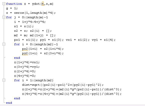
\( \begin{align*} \dot{x_1} &= v_{x1} \\ \dot{v_{x1}} &= \frac{gm_2(x_2-x_1)}{((x_2-x_1)^2+(y_2-y_1)^2)^{3/2}}\\ \dot{y_1} &= v_{y1} \\ \dot{v_{y1}} &= \frac{gm_2(y_2-y_1)}{((x_2-x_1)^2+(y_2-y_1)^2)^{3/2}}\\ \dot{x_2} &= v_{x2} \\ \dot{v_{x2}} &= \frac{gm_1(x_1-x_2)}{((x_1-x_2)^2+(y_1-y_2)^2)^{3/2}}\\ \dot{y_2} &= v_{y2} \\ \dot{v_{y2}} &= \frac{gm_1(y_1-y_2)}{((x_1-x_2)^2+(y_1-y_2)^2)^{3/2}} \end{align*}\)

Using this system of equations, we created a function ydot which gives us the trajectory of our bodies in motion. We expanded our code to work for any amount of bodies. So, when given our initial conditions we can get the rate of change of the bodies.

ydot

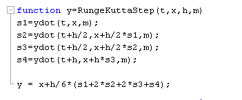
Now that we have established our ydot we need to use an approximation method that will give us very little error. We chose to use the Runge-Kutta Method of order four. Once again we expanded our code to work for any amount of bodies. The formulas for Runge-Kutta \(w_{i+1}, s_1, s_2, s_3, s_4\) as they are given in the book are found here:

Runge-Kutta

We then changed the given code for eulerstep and made it use the Runge-Kutta method.

Updated Code

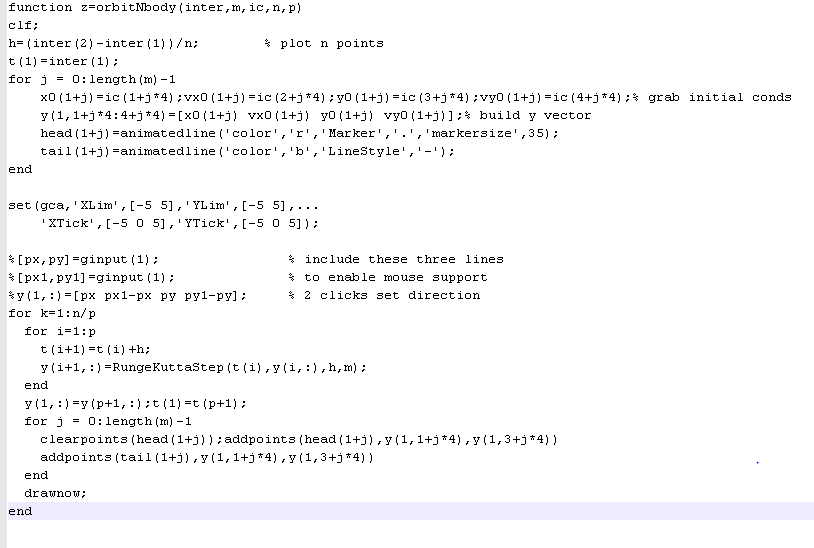
Once we put the proper arguments into orbitNbody we can see how these 2 bodies are behaving. Argument: orbitNbody([0 100],[0.03 0.3],[2 0.2 2 -0.2 0 -0.02 0 0.02],10000,5)

Problem 10a

We now turned our attention to a three-body problem. Now there are four more differential equations that need to be considered to give a total of 12.

\( \begin{align*} \dot{x_1} &= v_{x1} \\ \dot{v_{x1}} &= \frac{gm_2(x_2-x_1)}{((x_2-x_1)^2+(y_2-y_1)^2)^{3/2}} + \frac{gm_3(x_3-x_1)}{((x_3-x_1)^2+(y_3-y_1)^2)^{3/2}}\\ \dot{y_1} &= v_{y1} \\ \dot{v_{y1}} &= \frac{gm_2(y_2-y_1)}{((x_2-x_1)^2+(y_2-y_1)^2)^{3/2}} + \frac{gm_3(y_3-y_1)}{((x_3-y_1)^2+(y_3-y_1)^2)^{3/2}}\\ \dot{x_2} &= v_{x2} \\ \dot{v_{x2}} &= \frac{gm_1(x_1-x_2)}{((x_1-x_2)^2+(y_1-y_2)^2)^{3/2}} + \frac{gm_3(x_3-x_2)}{((x_3-x_2)^2+(y_3-y_2)^2)^{3/2}}\\ \dot{y_2} &= v_{y2} \\ \dot{v_{y2}} &= \frac{gm_1(y_1-y_2)}{((x_1-x_2)^2+(y_1-y_2)^2)^{3/2}} + \frac{gm_3(y_3-y_2)}{((x_3-x_2)^2+(y_3-y_2)^2)^{3/2}}\\ \dot{x_3} &= v_{x3} \\ \dot{v_{x3}} &= \frac{gm_1(x_1-x_3)}{((x_1-x_3)^2+(y_1-y_3)^2)^{3/2}} + \frac{gm_2(x_2-x_3)}{((x_2-x_3)^2+(y_2-y_3)^2)^{3/2}}\\ \dot{y_3} &= v_{y3}\\ \dot{v_{y3}} &= \frac{gm_1(y_1-y_3)}{((x_1-x_3)^2+(y_1-y_3)^2)^{3/2}} + \frac{gm_2(y_2-y_3)}{((x_2-y_3)^2+(y_2-y_3)^2)^{3/2}} \end{align*}\)

Since we extended our code to be able to take any number of bodies, all we needed to change was our input argument. Now there are three objects that have forces that act on the other two. Changing the input we can see how the three bodies behave. Argument:orbitNbody([0 200],[0.03,0.3,0.03],[2 0.2 2 -0.2 0 0 0 0 -2 -0.2 -2 0.2],10000,15)

Problem 10b

The next task was to make a slight change to the velocity of x1 (by +.0001) and see what the resulting trajectories were. The slightly different argument becomes: orbitNbody([0 200],[0.03,0.3,0.03],[2 0.20001 2 -0.2 0 0 0 0 -2 -0.2 -2 0.2],10000,15)

One body flies off the screen after about two revolutions while the other two start spiraling out of control. Clearly slight perturbations of the initial conditions have drastic affects on the trajectories of the bodies.

Problem 11a

Still using a three-body system we now want to consider C. Moore's discovery of the figure-eight orbit. The three bodies all have equal mass and chase each other along a single figure-eight loop. By once again only changing our input argument we can see the behavior of this orbit. Argument: orbitNbody([0 100],[1,1,1],[-0.970 -0.466 0.243 -0.433 0.970 -0.466 -0.243 -0.433 0 0.932 0 0.866],10000,15)

Problem 11b

Now we want to see if changing the third body's velocity by small values will make the three bodies break their figure-eight orbit.

Adding 10^-1 to the velocity of the third body gives a new velocity of 1.032.

For 10^-1 the figure-eight pattern does not persist. It starts moving to the right.

Adding 10^-2 :

For 10^-2 the figure-eight pattern deviates slightly from the original pattern.

Adding 10^-3 :

For 10^-3 the bodies are barely deviating from the original pattern, but it is still slightly noticable that the lines are getting thicker as time progresses.

Adding 10^-4 :

At this point the three-bodies are keeping the figure-eight pattern. It is very difficult to even see the lines getting thicker.

Adding 10^-5 :

Now there is no visible difference between this pattern and the original. This must mean that the error is so small that it is negligible.

3D Three Body Problem

We have adapted our program to be able to model a three-dimensional three body problem. The code for the three dimensional N body problem is Here

This code uses the differential equations: FILL IN HERE

Using the initial conditions input into the program orbitNbody3D([0 200],[0.03,0.3,0.03],[2 0.2 2 -0.2 0 0 0 0 0 0.01 0 -0.01 -2 -0.2 0 0 -2 0.2],10000,15), the modeled motion of the objects was:

It can be seen that the objects are orbiting each other, but the system is drifting upwards.

Error in the Three Body Problem

When writing our 3 body problem code, we incountered an error where the figure 8 system drifted upward:

We believe this error was caused in an older version of our code where we found each body's position as its own vector instead of solving the system as one vector. When solving it as individual vectors, the positions of the bodies when they were approximated were based off of the position in the previous time stem instead of using the most current position of the planets. This caused a small amount of error in the figure 8 problem that continued to be propogated each step so the planets ended up drift upwards. When the whole system is one vector, the positions are all calculated using the information found for the other planets in the same step, preventing this error from occuring.