This project explores the mathematics behind the global positioning system (GPS), a network which uses the position data received from satellites orbiting earth, and the time taken to receive a signal from one satellite to the receiver on earth to caclulate the \(x, y, z\) coordinates of said earthbound receiver.
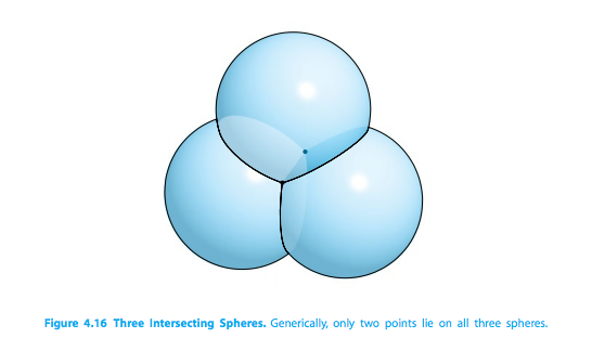
The idea is to draw \(n\) spheres around your \(n\) orbiting satellites, with \(x, y, z\) position \((A_{i},B_i, C_i)\) for \(i = \{1,2,...,n\}\). The case of \(n = 3\) is shown below. Notice how 3 spheres in 3d space intersect at most only 2 points (if all the spheres are different).
for \(x, y, z,\) and \(d\), where \(c\) is the speed of light \(\approx\) 299792.458 km/sec. In parts 1 and 2, we solve this system for \(n = 4\) using a multivariate Newton's method and then the quadratic formula. In the later parts, we examine an ill-conditioned case where the satellites are very close together and also where we increase \(n\) and so have more equations than unknowns. We will then explore how the error in calculated coordinates decreases with increasing \(n\). You can view the detailed project specs here.
We first begin by examining the case of 4 satellites with \((A, B, C)\) coordinates
| Satellite/\(i\) | \(x\)-position/\(A_i\) (km) | \(y\)-position/\(B_i\) (km) | \(z\)-position/\(C_i\) (km) | transmission time/\(t_i\) (s) |
|---|---|---|---|---|
| 1 | 15600 | 7540 | 20140 | 0.07074 |
| 2 | 18760 | 2750 | 18610 | 0.07220 |
| 3 | 17610 | 14630 | 13480 | 0.07690 |
| 4 | 19170 | 610 | 18390 | 0.07242 |
Thus we want to solve (1) for \(i = \{1,2,3,4\}\) using a multivariate Newton's to be sure that our \((x,y,z,d) = (-41.77271, -16.78919, 6370.0596, -.003201566)\). Attached here is our MATLAB code, and below is an example run of this code. Newton's method took 4 iterations to converge to the answer with an initial guess of (0, 100, 6400, 0.0001).

We started by foiling out the equations of 4.38 and then subtracting the second, third and fourth equations from the first. This gave us three seperate equations which had known coefficients for variables \(x,y,z,d\) and constant terms. This allowed us to make vectors of the coefficients and constant terms. Vectors
In order to get \(x\) in terms of \(d\) we solved the determinant equation given in the reality check. Then we did the same for \(y\) and \(z\). The key here was to structure the columns of the matrix in a way that when we took the determinant we were left with only \(x, y,\) or \(z\), and \(d\) as our variables. In terms of d
By plugging these new equations for \(x\), \(y\) and \(z\) back into 4.38, foiling, and then combining like terms we get a quadratic with respect to \(d\). This can obviously be solved using the quadratic formula.
Once we solve the quadratic formula, we will get solutions for \(d\). One will be the correct solution that we want from Part 1. The other will be far enough off that we can disregard it. In terms of our code, the first root is the correct value of \(d\). We can then plug in the correct root back into the equations of \(x,y,z\) in terms of \(d\) to get the reciever position. Part 2 Quadratic
The result of solving the quadratic and plugging in the solutions is Part 2 Result
The complete, compiled code for part 2 is here: Part 2 Code
In this part of the project, we were interested in how the seemingly slightest discrepancies in transmission time values \(t\) could drastically changed the calculated coordinated values on earth. Since we are working with spheres, we define our satellite positions via spherical coordinates \((\rho, \theta, \phi)\), where
\(\begin{align*} A_i &= \rho\cos\phi_{i}\cos\phi_{i}\\ B_i &= \rho\cos\phi_{i}\sin\phi_i\\ C_{i}&= \rho\sin\theta_i \end{align*}\)
We arbitarily chose \(\phi\) values between \([0, \frac{\pi}{2}]\) and \(\theta\) between \(\left[0,2\pi\right]\), and had \(\rho = 26570\) km.
\(\begin{align*} \phi &= \left[\frac{2\pi}{5}, \frac{\pi}{3}, \frac{\pi}{7}, \frac{\pi}{6}\right]\\ \theta &= \left[\frac{3\pi}{4}, \frac{\pi}{4}, \frac{5\pi}{3}, \frac{7\pi}{6}\right] \end{align*}\)
With these values and an initial guess of \([0, 100, 6400, .0001]\), our Newton's method converged to the exact solution of roughly (0, 0, 6370, .0001). We next wrote a program to find the error caused by varying each \(t\) entry by \(\pm 10^{-8}\). Out of the 16 possible combinations, we found which gave us the highest error magnification factor (emf), given by the ratio
\(\begin{equation*} emf = \frac{||(\Delta x, \Delta y, \Delta z)||_{\infty}}{c||\Delta t_{i}||_{\infty}} \end{equation*}\)
We found that with 4 satellites, the greatest position error was about .03007 km, and the greatest error magnification factor was given by about 10.029, with the \(t\) perturbation combination shown below.

The code for this can be viewed here. We also compared how much each individual \(t\) value affected the calculated position by varying each \(t\) value separately while holding the others fixed. Our results are summarized in the table below.
| Perturbation (s) | \(t_1 + 10^{-8}\) | \(t_2 + 10^{-8}\) | \(t_3 + 10^{-8}\) | \(t_4 + 10^{-8}\) |
|---|---|---|---|---|
| Max Position Error (km) | 0.01179 | 0.00845 | 0.00371 | 0.00659 | Max EMF | 3.9319 | 2.8178 | 1.2388 | 2.1966 |
This next part viewed the ill-conditioned problem: what happens when 4 satellites are bunched too closely together? We considered "too close" to be both \(\phi\) and \(\theta\) values within 5% of each other. We used the same code as in part 4, but this time with the angles
\(\begin{align*} \phi_i &= \left[\frac{\pi}{3}, \frac{\pi}{3} + \frac{\pi}{80}, \frac{\pi}{3} - \frac{\pi}{80}, \frac{\pi}{3} + \frac{\pi}{100}\right]\\ \theta_i &= \left[\frac{5\pi}{6} - \frac{\pi}{22}, \frac{5\pi}{6} + \frac{\pi}{22}, \frac{5\pi}{6}+\frac{\pi}{20}, \frac{5\pi}{6} - \frac{\pi}{21}\right] \end{align*}\)
With these close satellites, our solution still converged to the same vector (0, 0, 6370, .0001), but this time we saw a huge jump in both our maximum position error and maximum emf, from about 0.03007 km to 4.6445 km, and from 10 to roughly 1550, respectively. Also notice that it had to run through the maximum iterations because the tolerance used in part 4 is too low for part 5, i.e. this part is less accurate.

In the final part of the project we were to compare the results from the cases of 4 unbunched satellites, 4 bunched, and the addition of more satellites to determine the optimal configuration. Our group chose to write code which would output the maximum position error and the maximum magnification factor for 4-12 satellites individually. Our results are summarized in the table below:
| # of satellites | Max Position Error (km) | Max EMF | \(t\) combination \((\pm 10^{-8})\) s |
|---|---|---|---|
| 4 | 0.03007 | 10.0289 | +,-,+,- |
| 5 | 0.00889 | 2.9549 | +,+,-,-,- |
| 6 | 0.00823 | 2.7439 | +,+,-,-,-,+ |
| 7 | 0.00828 | 2.7629 | +,+,-,-,-,+,+ |
| 8 | 0.00814 | 2.7160 | +,+,-,-,-,+,+,- |
| 9 | 0.00838 | 2.7938 | +,+,-,-,-,+,+,-,+ |
| 10 | 0.00791 | 2.6382 | +,+,-,-,-,+,+,-,+,+ |
| 11 | 0.00808 | 2.6954 | +,+,-,-,-,+,+,-,-,+,+ |
| 12 | 0.00735 | 2.4828 | +,+,-,-,-,+,+,-,+,+,+,- |
Because any number of satellites greater than 4 results in more equations than unknowns, our code uses a Gauss-Newton method to solve the system. You can check the code out here. (Give it a few seconds to run.)
From the table, it is clear that 12 satellites provides the lowest position error and condition number. However, 12 satellites tracking one target is not very practical. Once you have \(n = 5\), adding any more only improves your position error on the order of one ten-thousandth of a kilometer, or one tenth of a meter. Thus, if the cost of additional satellites is considered, 5 satellites is probably enough to secure accuracy and cost-efficiency. Additionally, when we added more satellites we kept them far away from each other. So, with any number of satellites used, even 12, you want to make sure they are sufficiently far enough away, or the errors seen in part 5 will most likely reappear.