Image Compression
Harnam Arneja
My Home Page.
Math 447 Home Page.
Overview
Compression of data allows for data to transfer quickly between two sources and is based on
numerical methods. Specifically, compression requires the usage of a Discrete Cosine Transformation,
often abbreviated DCT, which is a finite sequence of points represented by cosine functions with
different frequencies. For more information on DCTs, visit the
wikipedia page.
Also, quantization can be used to apply a filter, such a low pass frequency or high pass frequency, which
will allow less bits to store data. In order to compression an image, such as in the JPEG format,
quantization and discrete cosine transform is used. When implementing image compression in code, the
image is indexed in terms of 8 x 8 blocks in which the data is compressed and then displayed.
The sections below discuss the implementation and results of using DCT and JPEG compression.
For this project, images were read into MatLab by using the built in imread function which
saves the color values in red, green, and blue at each pixel location. The values of each color
range from [0,255] by integers. This project utilizes
transformations and quantizations on this color values which allows for digital compression.
The main code can be downloaded and run in MatLab.
In this section, a color image was converted to gray scale and then was compressed by DCT and quantization. Here is the code
used to convert color images to gray scale. The discrete cosine transform matrix can be found by the following equations:
\begin{align}
C_{ij} &= \frac {\sqrt{2}}{\sqrt{n}} \ a_i \ cos\left(\frac{i(2j+1) \pi}{2n} \right) \\
\\
a_i &= \begin{cases}
1/ \sqrt{2} &\text{if } i=0, \\
1 &\text{if } i=1,...,n-1 \\
\end{cases}
\end{align}
Note that the C matrix listed above is an orthogonal matrix which means that the transpose, \( C^T \), is the same as the inverse, \(C^{-1} \). Image compression
typically indexes through the image in 8 x 8 pixel blocks which makes \(n=8\) for the DCT.
After the cosine transformation is complete, the color data is then centred around 0 by subtracting 128. Then,
the data is quantized by multiplying on the right by \(Q^{-1}\), rounding to the nearest integer, and then multiplying
on the right by \(Q\). It is important to multiply on the same side as matrices are generally non-commutative. This process
is which data is lost which allows for the image compression. There are various methods for the quantization matrix, Q, and the
first one used was \(Q_{linear}\) which is shown below. The parameter p is known as the loss parameter which allows for less data
to be stored but comes at the cost of a lower quality image.
\begin{align}
Q_{linear}= p \left[ {\begin{array}{cccccccc}
8 & 16 & 24 & 32 & 40 & 48 & 56 & 64 \\
16 & 24 & 32 & 40 & 48 & 56 & 64 & 72 \\
24 & 32 & 40 & 48 & 56 & 64 & 72 & 80 \\
32 & 40 & 48 & 56 & 64 & 72 & 80 & 88 \\
40 & 48 & 56 & 64 & 72 & 80 & 88 & 96 \\
48 & 56 & 64 & 72 & 80 & 88 & 96 & 104\\
56 & 64 & 72 & 80 & 88 & 96 & 104 & 112 \\
64 & 72 & 80 & 88 & 96 & 104 & 112 & 120 \\
\end{array} } \right]
\end{align}
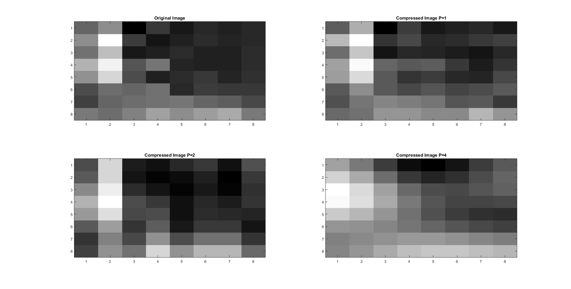
The results of using linear compression on a gray scaled image are shown below for different
cases of \(p={1,2,4}\). To better analyze the difference, the graphs show an 8 x 8 section of
the image.
Figure 1: Linear Quantization 8 x 8
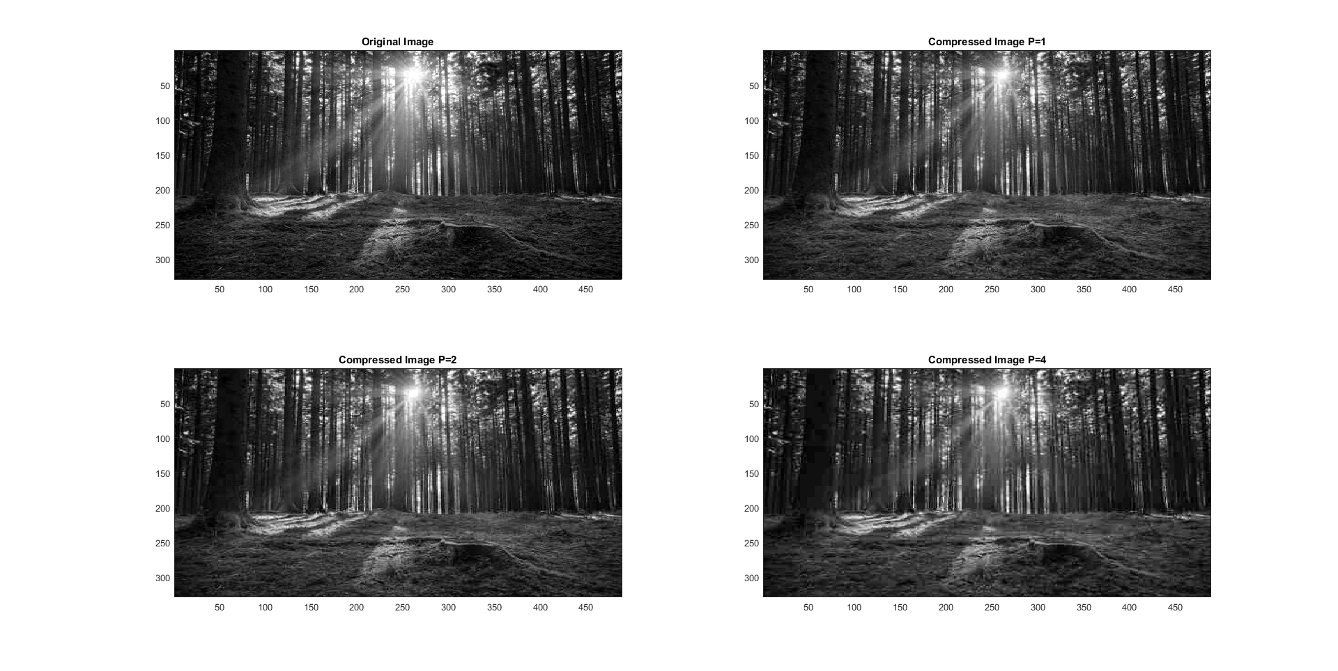
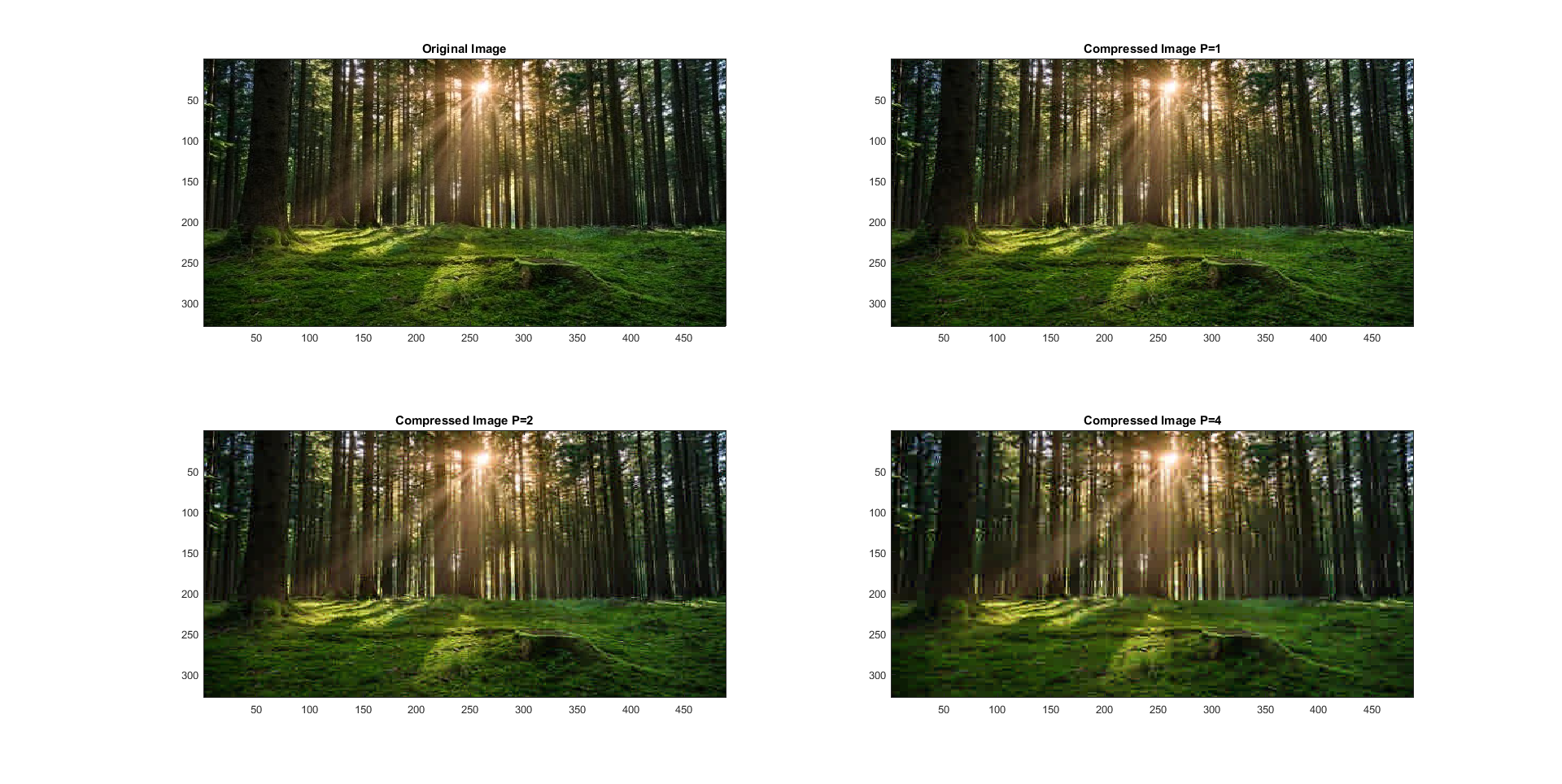
Then, the same method used to create figure 1 was implemented across the entire object.
The results of the linear quantization and compression is shown below in figure 2:
Figure 2: Linear Quantization Complete Image

This section involves compression of a grayscale image using the JPEG
recommended matrix as shown below.
\begin{align}
Q_{JPEG}= p \left[ {\begin{array}{cccccccc}
16 & 11 & 10 & 16 & 24 & 40 & 51 & 61\\
12 & 12 & 14 & 19 & 26 & 58 & 60 & 55 \\
14 & 13 & 16 & 24 & 40 & 57 & 69 & 56 \\
14 & 17 & 22 & 29 & 51 & 87 & 80 & 62 \\
18 & 22 & 37 & 56 & 68 & 109 & 103 & 77 \\
24 & 35 & 55 & 64 & 81 & 104 & 113 & 92 \\
49 & 64 & 78 & 87 & 103 & 121 & 120 & 101 \\
72 & 92 & 95 & 98 & 112 & 100 & 103 & 99 \\
\end{array} } \right]
\end{align}
The results of JPEG compression are shown for different values of \(p={1,2,4}\) below in figure 3. Comparing the two cases, it is clear
that the JPEG quantization results in a more clear image for the same values of p.
Figure 3: JPEG Quantization 8 x 8
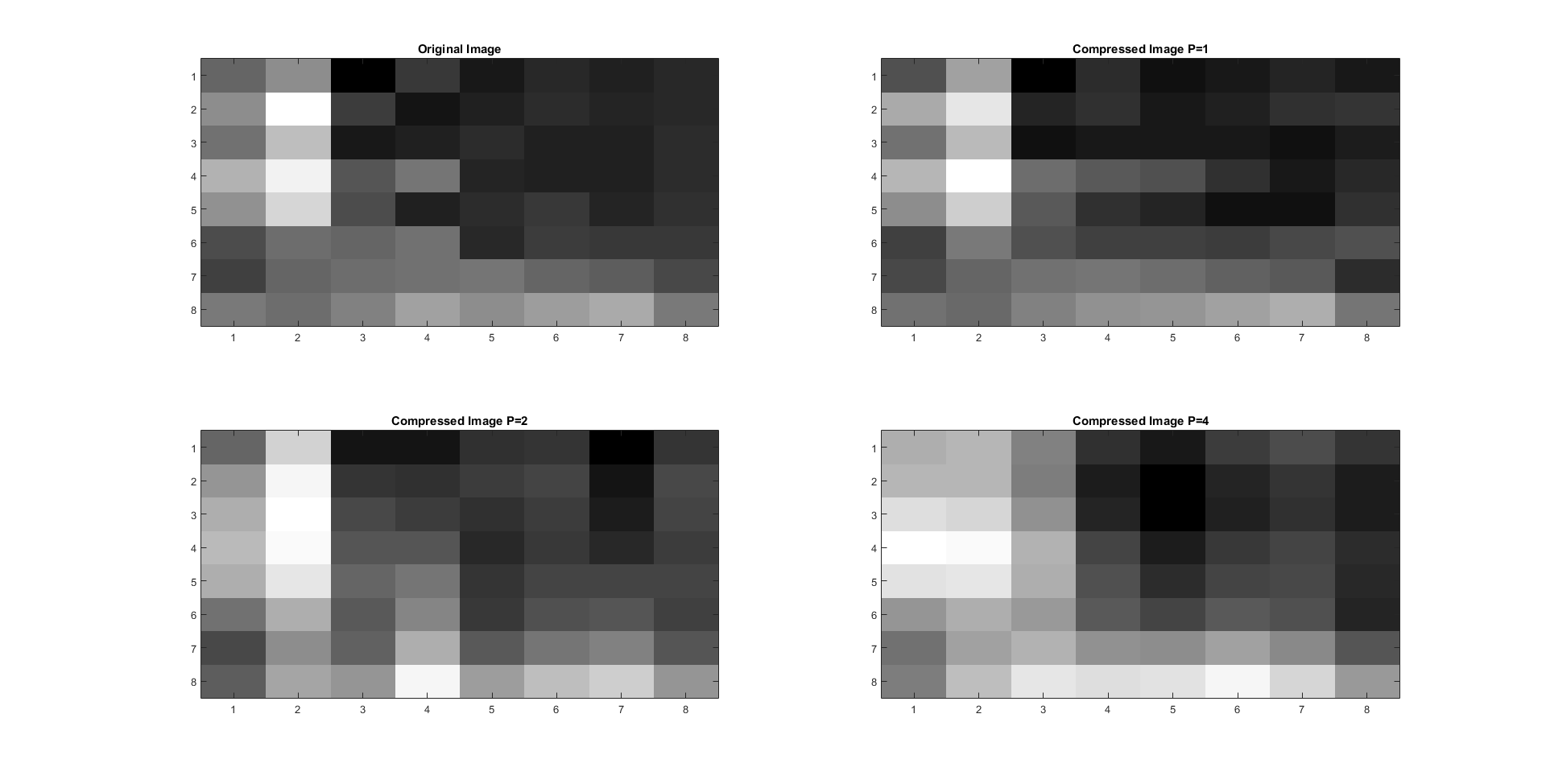
Figure 4: JPEG Quantization
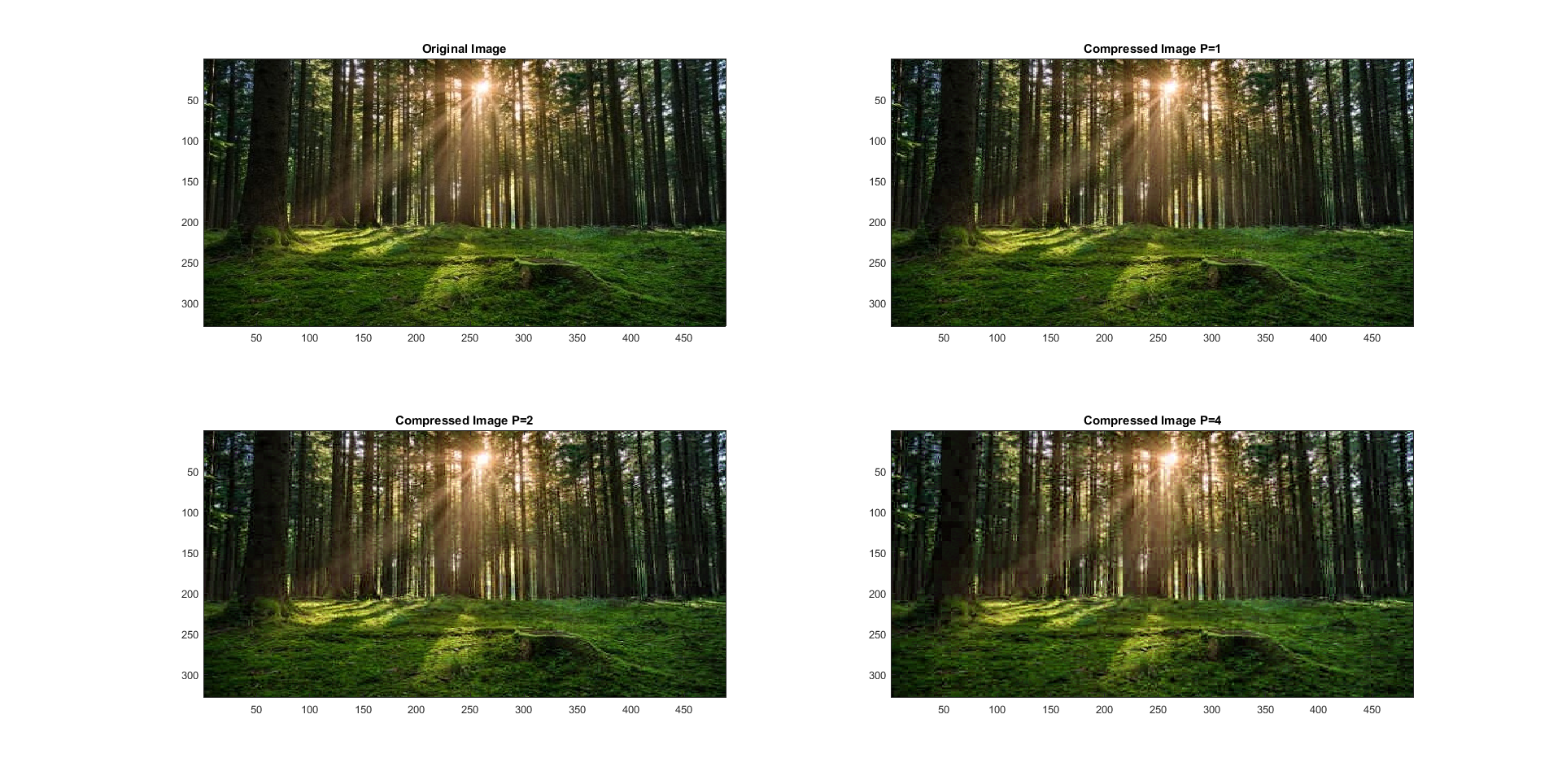
Color linear quantization repeats the linear quantization and compression process to part one but for all three of the color variables:
red, green, and blue. The results are shown below in figures 5 and 6.
Figure 5: Linear Quantization in Color 8 x 8
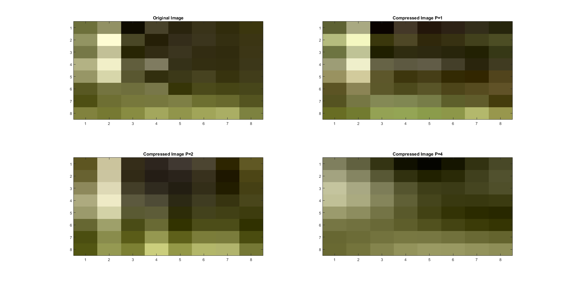
Figure 6: Linear Quantization in Color
The luminance color system creates variables YUV, in which Y is defined
as a color combination of red, green, and blue and then U and V are defined as color
differences between Y and red, and Y and blue. The formulas are shown below.
\begin{align}
Y &= 0.299R +0.587G + 0.144B \\
U &= B-Y \\
V &= R-Y\\
\end{align}
Different quantization matrices are used on the corresponding YUV variables. For the Y variable, the JPEG recommended matrix is used but for
the U and V variables the \(Q_{color}\) matrix is used and is shown below.
\begin{align}
Q_{color}= p \left[ {\begin{array}{cccccccc}
17 & 18 & 24 & 47 & 99 & 99 & 99 & 99 \\
18 & 21 & 26 & 66 & 99 & 99 & 99 & 99 \\
24 & 26 & 56 & 99 & 99 & 99 & 99 & 99 \\
47 & 66 & 99 & 99 & 99 & 99 & 99 & 99 \\
99 & 99 & 99 & 99 & 99 & 99 & 99 & 99 \\
99 & 99 & 99 & 99 & 99 & 99 & 99 & 99 \\
99 & 99 & 99 & 99 & 99 & 99 & 99 & 99 \\
99 & 99 & 99 & 99 & 99 & 99 & 99 & 99 \\
\end{array} } \right]
\end{align}
The results of the luminance compression are shown below in figures 6 and 7:
Figure 6: Luminance 8 x 8
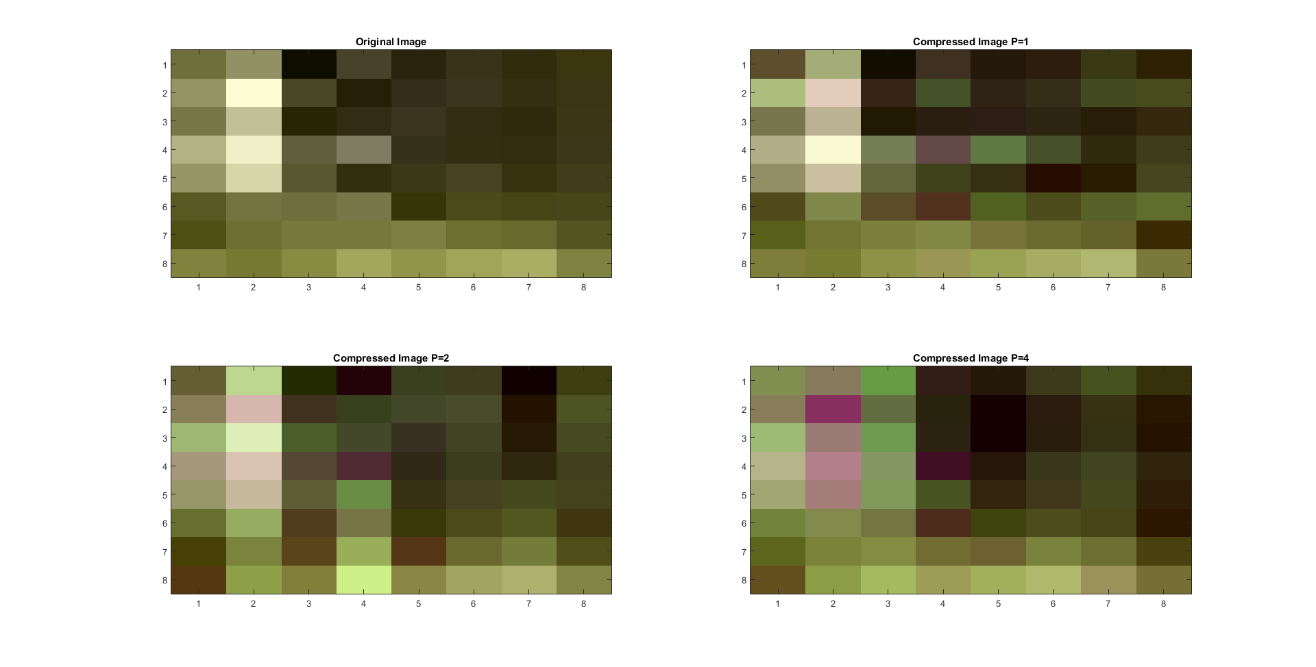
Figure 7: Luminance