
Professor, George Mason University — dwilsonb@gmu.edu — Last updated: 08 April 2021
Download macro here
This page contains documentation for the SPSS macro MetaAnal.sps. This macro performs inverse-variance weighted meta-analysis within SPSS and is a complete re-write of the prior three macros MeanES.sps, MetaF.sps, and MetaReg.sps. You can download the original macros here. The macro performs both fixed-effect and random-effects models and includes options for subgroup analysis and regression-based moderator analysis.
At a minimum, this macro requires an effect size and inverse variance weight. Furthermore, the macro assumes that you have already applied any needed transformations to analyze the effect size. For example, you have converted odds ratios to logged odds ratios, risk ratios to logged risk ratios, correlations (r) to Fisher’s zr, and proportions to logits.
In addition to a fixed-effect model, the macro can fit random-effects models based on eight different estimators for the random effects variance component (τ2).
To use these macros, you must perform your analyses from a syntax window rather than through the GUI system (i.e., the pull-down menus). After downloading and unzipping the MetaAnal.sps macro, place it in a folder that makes sense within your system. For example, I placed it in the user “david”’s "Documents_Macros" folder in the example below. To use, you must first initialize the macro with the `include’ syntax statement. You only need to do this once during any given SPSS session, as illustrated below.
include "C:\Users\david\Documents\SPSS_Macros\MetaAnal.sps" .After running this command, you should see the following (or something similar) in the SPSS’s output window. This output indicates that the macro was successfully read by SPSS and is now ready to use.
    *--------------------------------------------------------------
    *' SPSS Macro for Performing Meta-analysis
    *' Written by David B. Wilson
    *' See http://mason.gmu.edu/dwilsonb/ma.html for documentation
    *' Version 2021.04.06
    *' License:
    *'   CC Attribution-Noncommercial-Share Alike 4.0 International
*-------------------------------------------------------------- .A basic meta-analysis using macro defaults with no moderator variables is run by specifying the variable name in the active SPSS dataset that contains the effect size and the inverse variance weight, as shown below.
    metaanal es = varname
            /w = varname .
The default model is a random-effects model using the restricted maximum likelihood estimator. You can run other model types via the /model = option. For example, the code below produces a fixed-effect (or common-effect) model.
    metaanal es = varname
            /w = varname
            /model = FE .
All model options are shown in the table below.
/model = |
Explanation |
|---|---|
FE |
Fixed (common) effect |
REML |
Restricted maximum likelihood (default) |
DL |
Dersimonian-Laird |
HE |
Hedges |
HS |
Hunter and Schmit |
SJ |
Sidik-Jonkman |
SJIT |
Sidik-Jonkman with iteraction |
ML |
Full-information maximum likelihood |
EB |
Empirical Bayes |
An optional specification is the /print = statement. This option enables you to transform results back into an original metric, such as an odds ratio or correlation. For example, /print = EXP exponentiates the mean effect size and 95% confidence interval. This option is useful for any effect size in the log form (i.e., logged odds ratio, logged risk ratio, logged incident rate ratio). All print options are shown in the table below.
/print = |
Explanation |
|---|---|
EXP |
Exponentiates results, converting |
| logged odds ratios, logged risk ratios, | |
| logged incident ratios, etc, back into | |
| their unlogged form | |
IVZR |
Inverse Fisher’s zr transformation; |
| converts zrs back into rs | |
PROP |
Inverse logit transformation; |
| converts logits back into proportions |
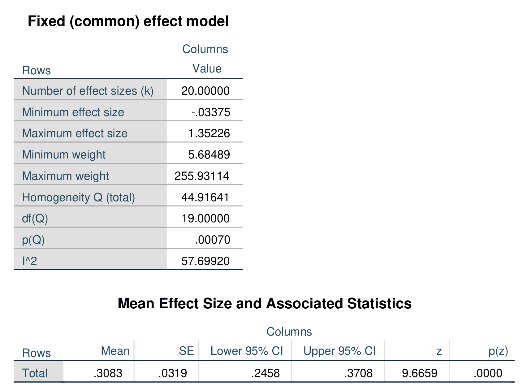
Sample output for a fixed-effect model and a random-effects model estimated via restricted maximum likelihood are shown below.
An example of output from the above command is shown below. In this example, the effect size is a standardized mean difference, specifically Hedges’ g.
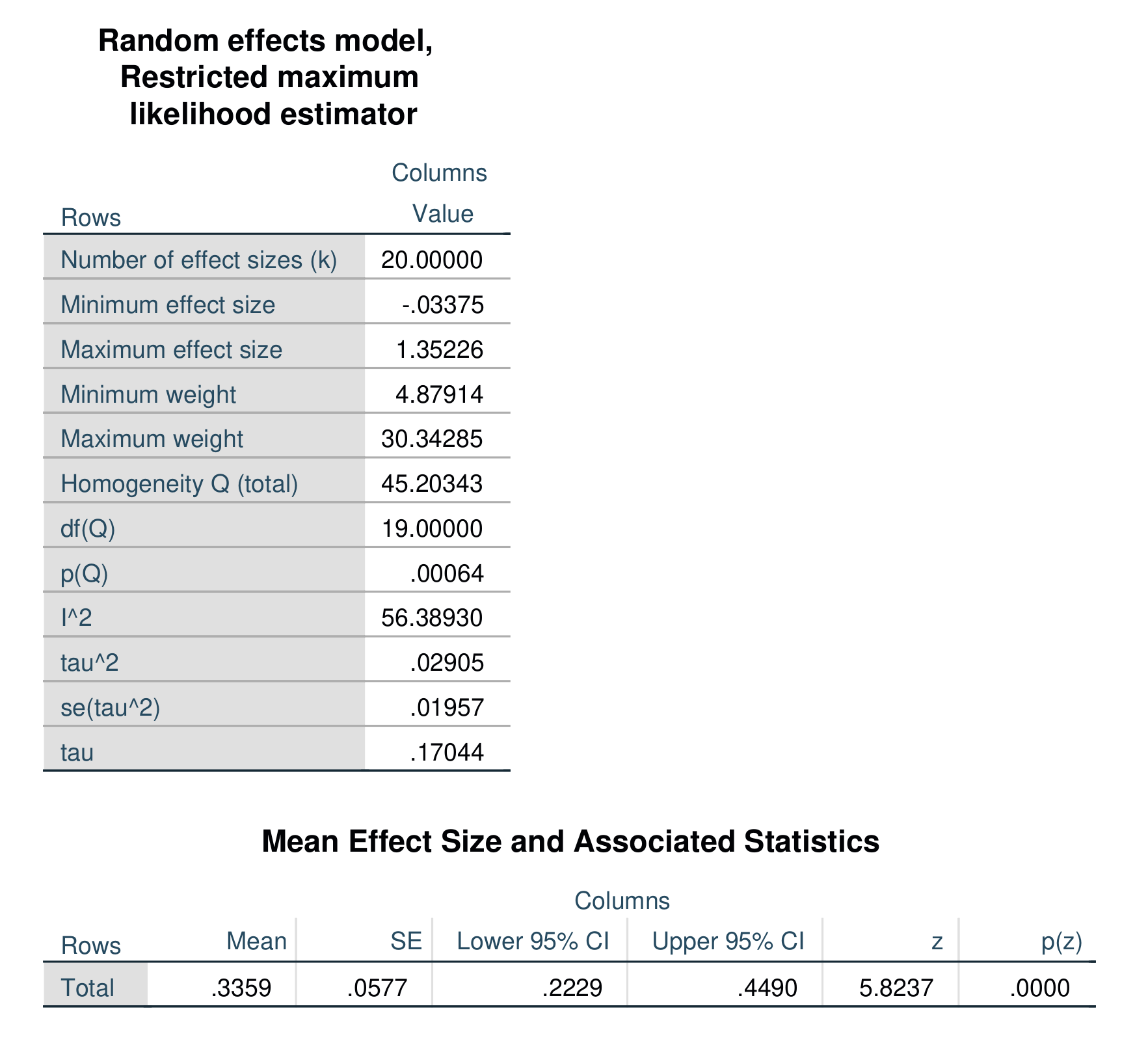
Re-running the above analysis as a random-effects model estimated via restricted maximum likelihood produces the following output.
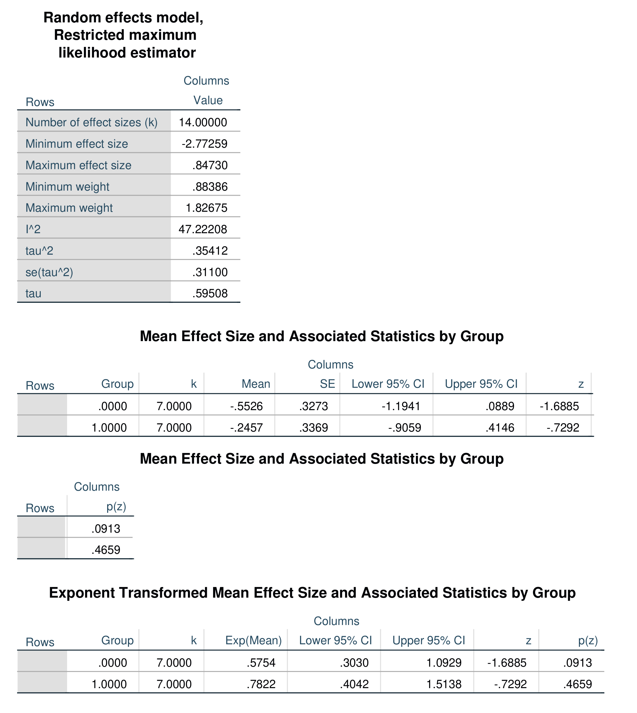
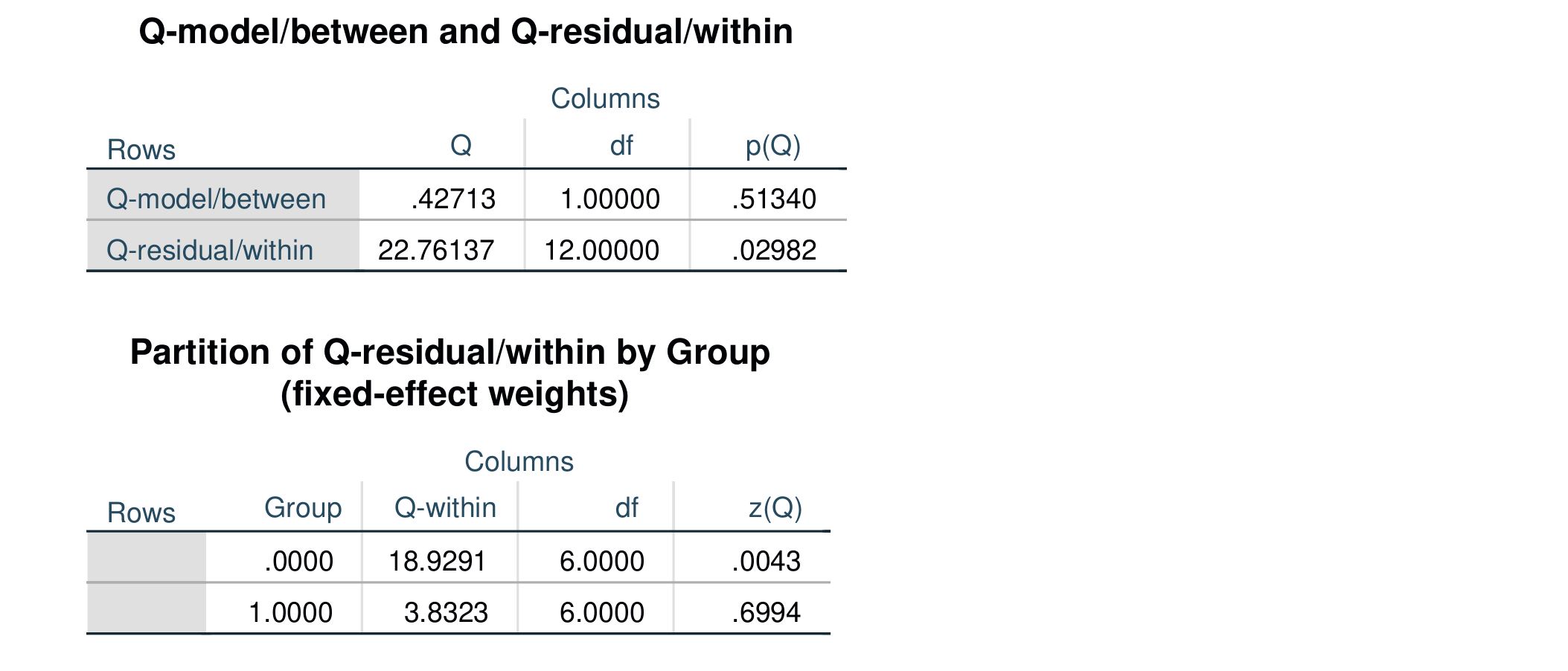
A common form of moderator analysis compares the mean effect size across subgroups defined by a categorical variable or factor. You can run this type of moderator analysis with this macro using the /group = specification. The variable specified must be categorical. Specifying a categorical moderator using this specification will produce a mean effect size for each category and associated statistics as well as a Q-test for the moderator that is analogous to an F-test from a oneway ANOVA. The latter is designated as Q-model/between in the output. An example of the syntax is shown below. The variable name for the effect size in this dataset is g, the variable name for the inverse variance weight is invw, and the categorical moderator variable is txtype.
    metaanal es = g
             /w = invw
             /group = txtype
             /model = REML .
An optional specification for subgroup moderator analysis is the /tau_unique = YES subcommand. Adding this will instruct the macro to compute a separate random effects variance component for each subgroup. The default is to use a common random effects variance component across groups. The syntax for the above example with this option specified is shown below.
    metaanal es = g
             /w = invw
             /group = txtype
             /model = REML
             /tau_unique = YES .
Note that print options also work for subgroup analyses.
Output for the above model is shown below.
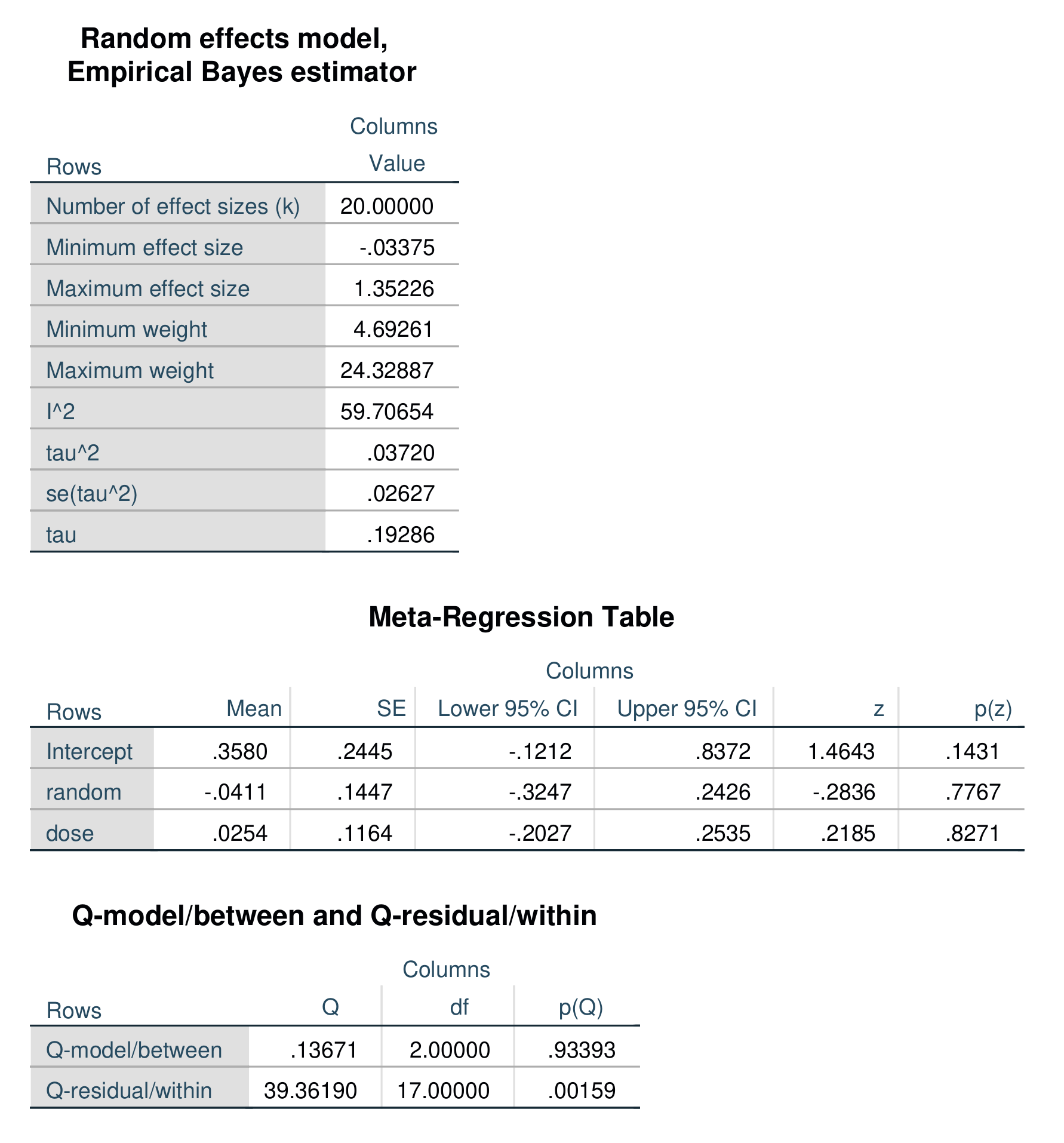
Regression-based moderator analysis, often called meta-regression, can be performed with the /ivs = specification. You can specify one or more independent variables. These can be binary, ordinal, or scaled variables. All of the /model options remain the same, but the /print subcommand has no effect and will be ignored if specified. The example below specifies two independent variables, txtype (a binary dummy-code), and dosage, a scaled variable. This syntax also specifies the Dersimonian-Laird random-effects estimator.
    metaanal es = g
             /w = invw
             /ivs = random dose
             /model = EB .
Output for the above model is shown below. In this model, random is a binary variable and dose is a three-level ordinal variable.
This macro is licensed under the Creative Commons Attribution-Noncommercial-Share Alike 4.0 International license link. The code that computes the random-effets variance components is based on code contained in Wolfgang Viechtbaur’s metafor package for R.
Last update 12 July 2021