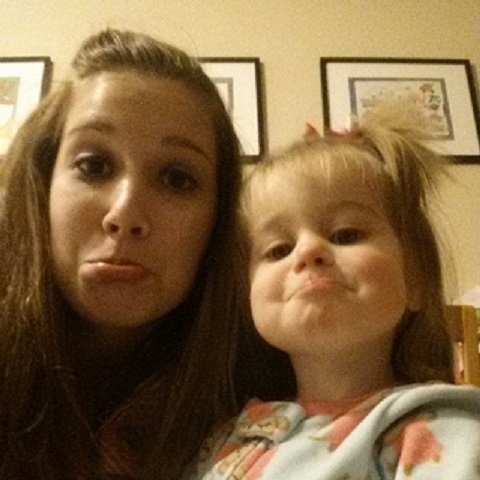

This project is to help us understand compression of files, there was a choice of audio or image files, and I went with image compression. This project focuses on DISCRETE COSINE TRANSFORM, or dct. This transform uses the cosine function to interpolate real computations. DCT is just taking a least squares model and having the following function:
Pn(t) = \(\frac{1}{\sqrt{\textit{n}}}\)y0+\(\frac{\sqrt{2}}{\sqrt{\textit{n}}}\) +\(\sum^{\textit{n}-1}_{\textit{k} = 1}\)ykcos\(\frac{\textit{k}(x\textit{t}+1)\pi}{2\textit{n}}\)
For image compression we are taking both the horizontal and vertical directions, since an image is 2 dimensional, but this is just applying DCT 2 times, in MATLAB is done by using the following command dct(dct(xb')') where xb is a matrix represents the picture, or part of a picture, that is imported into MATLAB. NOTE! When an image is imported into MATLAB, this is a 3-dimensional array, [m,n,a] where a is storing color or RGB, where R is in the first array, G is in the second array and B is in the third array.
Since we know by now that MATLAB likes to handle numbers in matrices, the above polynomial is represented in a matrix.
After we compress the image by using the dct function, we want to quantize all of the terms in the matrix. This means that MATLAB filters in a more selective way, by only allowing low filters to be saved because it means there is less memory being stored. For quantization, we used the round(y/Q ) function and this did the more selective filtering. The round( ) function makes numbers that are stored in the matrix to be rounded to the nearest integer. This makes a lot of numbers round to zero, as seen later in the project, which means there is not as much memory being used to store information. y is a matrix that has been transformed, and Q = p * some matrix. In this project we either used Q = p*8.hilb(8), where hilb(8) is a hilbert matrix. Or we used JPEG suggest matrix. Below is the JPEG suggest matrix that will be used in the code:
(11.25) QY = p \(\pmatrix{ 16 & 11 & 10 & 16 & 24 & 40 & 51 & 61 \cr 12 & 12 & 14 & 19 & 26 & 58 & 60 & 55 \cr 14 & 13 & 16 & 24 & 40 & 57 & 69 & 56 \cr 14 & 17 & 22 & 29 & 51 & 87 & 80 & 62 \cr 18 & 22 & 37 & 56 & 68 & 109 & 103 & 77 \cr 24 & 35 & 55 & 64 & 81 & 104 & 113 & 92 \cr 49 & 64 & 78 & 87 & 103 & 121 & 120 & 101 \cr 72 & 92 & 95 & 98 & 112 & 100 & 103 & 99}\)
For most of this project we do compression in either grayscale or RGB, red-blue-green. However, in the last part of this project was compressing an image in luminance. All this is doing is transforming RGB to YUV. I will define 7 items in the following paragraph that are used for YUV:
The next 4 are used for during image compression:
Y = 0.299R + 0.587G +0.144B
U = B - Y
V = R - Y
QC = p \(\pmatrix{ 17 & 18 & 24 & 47 & 99 & 99 & 99 & 99 \cr 18 & 21 & 26 & 66 & 99 & 99 & 99 & 99 \cr 24 & 26 & 56 & 99 & 99 & 99 & 99 & 99 \cr 47 & 66 & 99 & 99 & 99 & 99 & 99 & 99 \cr 99 & 99 & 99 & 99 & 99 & 99 & 99 & 99 \cr 99 & 99 & 99 & 99 & 99 & 99 & 99 & 99 \cr 99 & 99 & 99 & 99 & 99 & 99 & 99 & 99 \cr 99 & 99 & 99 & 99 & 99 & 99 & 99 & 99 \cr}\)
After the image is compressed we convert back to RGB by using the following equations:
B = U + Y
R = V + Y
G = \(\frac{\textit{Y} - 0.299\textit{R} - 0.114\textit{B}}{0.587}\)
Image compression is done the same way for the most part for all of the color scales, there just have to be translations to what you want to compress with.
In this part of the project I was to obtain a grayscale image of my choice, and use the imread command to import into MATLAB. I was lucky because my image was 480 x 480, which is a multiple of 8 so I did not have to resize my picture. The next paragraph explains the steps that were taken.
(a) Extract an 8 \(\times\) 8 pixel block using the MATLAB command, i.e. xb = x(81:88,81:88), and display the block with the imagesc command.
(b) Apply 2D-DCT.
(c) Quantize by using linear quantization with p = 1, 2, and 4. Printing out each of the YQ
(d) Reconstruct the block using the inverse 2D-DCT and compare the picture with the original picture. In this step I was to use the MATLAB commands colormap(gray) and imagesc(X, [0,255]).
(e) Then I was to carry out (a)-(d) for all 8 \(\times\) 8 blocks, and reconstiture the image in each case.
\(\star\) \(\star\)In the code for each of my section, I have commented what does what, i.e. Part B is in this part of the code since that was outlined in the book.\(\star\) \(\star\)
Here is the original image from above in the grayscale. project5grayscale.m, is the code that I used to make my picture in greyscale.
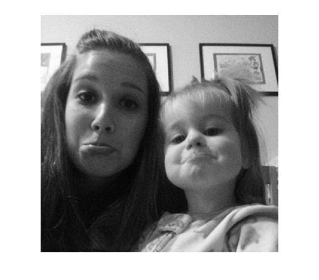
project5number3ad.m is the code that I used for the 8\(\times\)8 section that was done alone. Below is my original 8 \(\times\) 8 section from my picture(I think it is my eye in the picture, but I am not 100% sure):

And here are the p = 1, 2, and 4 pictures respectively. Followed by the Yq values.
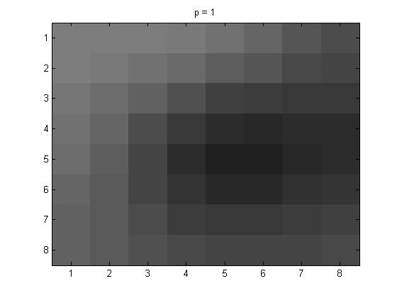
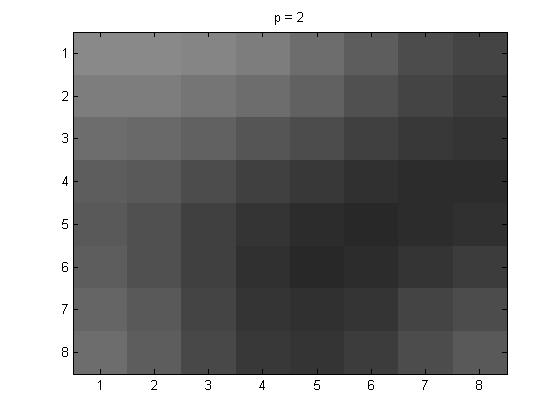
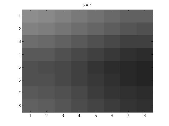
Next are the Yq values that I got for the different p values.
When p = 1, Yq = \(\pmatrix{ -50 & 9 & 2 & 0 & 0 & 0 & 0 & 0 \cr 6 & 1 & -1 & 0 & 0 & 0 & 0 & 0 \cr 4 & -1 & -1 & 0 & 0 & 0 & 0 & 0 \cr 0 & 0 & 0 & 0 & 0 & 0 & 0 & 0 \cr 0 & 0 & 0 & 0 & 0 & 0 & 0 & 0 \cr 0 & 0 & 0 & 0 & 0 & 0 & 0 & 0 \cr 0 & 0 & 0 & 0 & 0 & 0 & 0 & 0 \cr 0 & 0 & 0 & 0 & 0 & 0 & 0 & 0} \)
When p = 2, Yq = \(\pmatrix{ -25 & 4 & 1 & 0 & 0 & 0 & 0 & 0 \cr 3 & 1 & -1 & 0 & 0 & 0 & 0 & 0 \cr 2 & -1 & -1 & 0 & 0 & 0 & 0 & 0 \cr 0 & 0 & 0 & 0 & 0 & 0 & 0 & 0 \cr 0 & 0 & 0 & 0 & 0 & 0 & 0 & 0 \cr 0 & 0 & 0 & 0 & 0 & 0 & 0 & 0 \cr 0 & 0 & 0 & 0 & 0 & 0 & 0 & 0 \cr 0 & 0 & 0 & 0 & 0 & 0 & 0 & 0} \)
When p = 4, Yq = \(\pmatrix{ -12 & 2 & 0 & 0 & 0 & 0 & 0 & 0 \cr 2 & 0 & 0 & 0 & 0 & 0 & 0 & 0 \cr 1 & 0 & 0 & 0 & 0 & 0 & 0 & 0 \cr 0 & 0 & 0 & 0 & 0 & 0 & 0 & 0 \cr 0 & 0 & 0 & 0 & 0 & 0 & 0 & 0 \cr 0 & 0 & 0 & 0 & 0 & 0 & 0 & 0 \cr 0 & 0 & 0 & 0 & 0 & 0 & 0 & 0 \cr 0 & 0 & 0 & 0 & 0 & 0 & 0 & 0} \)
project5number3e.m is what was used to create the pictures as a whole. The pictures below are as follows: line (1): original grayscale, line (2): p = 1, p = 2, and p = 4.


For fun, I tried p = 100, and below is the image that I got,
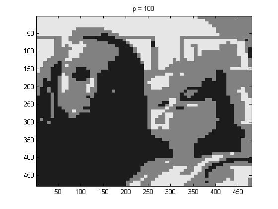
If you know what the original picture looks like you get the general shapes and gist of what the picture is supposed to look like. But had I not known what picture I was compressing I would not have guessed what this picture was.
In this part of the project I was to carry out Computer Problem 3, but quantize by the JPEG suggested matrix (11.25), defined in the introduction, with p = 1.
In this part of the project, for the 8 \(\times\)8 I used project5number4ad.m with p = 1, 2, and 4.
The pictures below are as follows for the 8\(\times\)8: line (1): original grayscale, line (2): p = 1, p = 2, and p = 4.
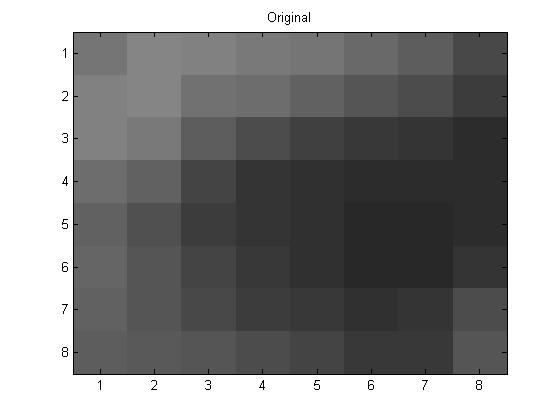
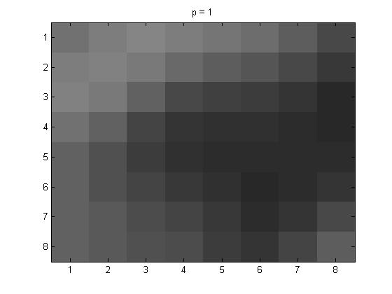
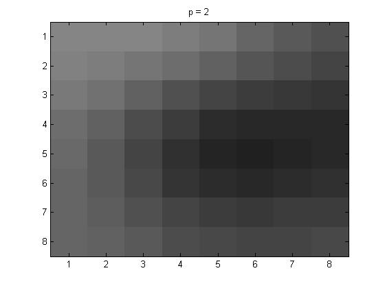
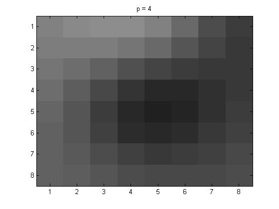
Next are the Yq values that I got for the different p values.
When p = 1, Yq = \(\pmatrix{ -25 & 13 & 4 & 0 & 0 & 0 & 0 & 0 \cr 8 & 3 & -3 & 1 & -1 & 0 & 0 & 0 \cr 7 & -2 & -2 & -1 & 0 & 0 & 0 & 0 \cr 0 & -1 & -1 & 0 & 0 & 0 & 0 & 0 \cr 0 & -1 & 0 & 0 & 0 & 0 & 0 & 0 \cr 0 & 0 & 0 & 0 & 0 & 0 & 0 & 0 \cr 0 & 0 & 0 & 0 & 0 & 0 & 0 & 0 \cr 0 & 0 & 0 & 0 & 0 & 0 & 0 & 0} \)
When p = 2, Yq = \(\pmatrix{ -12 & 7 & 2 & 0 & 0 & 0 & 0 & 0 \cr 4 & 1 & -1 & 0 & 0 & 0 & 0 & 0 \cr 4 & -1 & -1 & 0 & 0 & 0 & 0 & 0 \cr 0 & 0 & 0 & 0 & 0 & 0 & 0 & 0 \cr 0 & 0 & 0 & 0 & 0 & 0 & 0 & 0 \cr 0 & 0 & 0 & 0 & 0 & 0 & 0 & 0 \cr 0 & 0 & 0 & 0 & 0 & 0 & 0 & 0 \cr 0 & 0 & 0 & 0 & 0 & 0 & 0 & 0} \)
When p = 4, Yq = \(\pmatrix{ -6 & 3 & 1 & 0 & 0 & 0 & 0 & 0 \cr 2 & 1 & -1 & 0 & 0 & 0 & 0 & 0 \cr 2 & 0 & -1 & 0 & 0 & 0 & 0 & 0 \cr 0 & 0 & 0 & 0 & 0 & 0 & 0 & 0 \cr 0 & 0 & 0 & 0 & 0 & 0 & 0 & 0 \cr 0 & 0 & 0 & 0 & 0 & 0 & 0 & 0 \cr 0 & 0 & 0 & 0 & 0 & 0 & 0 & 0 \cr 0 & 0 & 0 & 0 & 0 & 0 & 0 & 0} \)
In this part of the project I used project5number4e.m, for the full picture, and I used p = 1, 2, 4 and 100, below are the pictures respectively:
But first as a reminder, here is the original photo in grayscale:

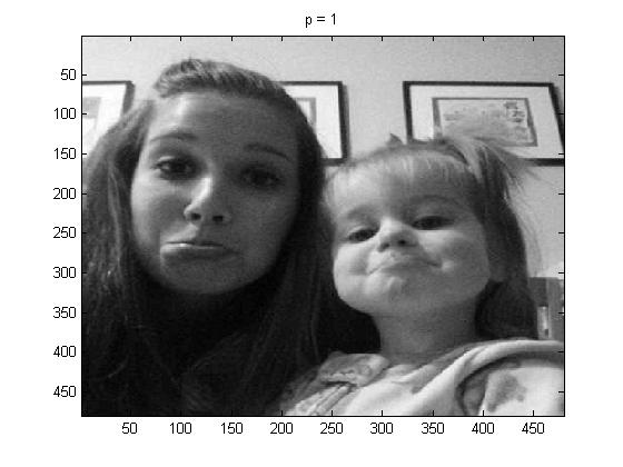
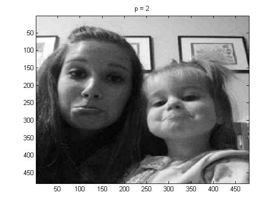

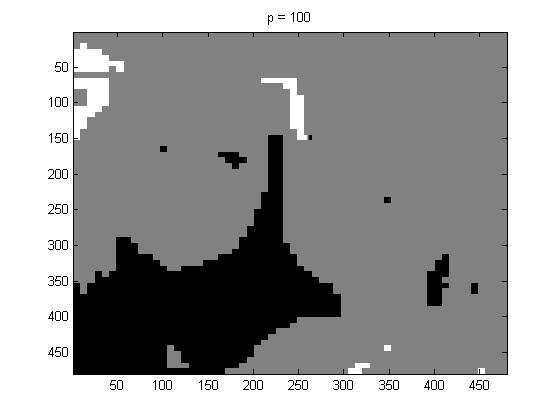
Again one can see that if we had not known what the original picture was, it would be really hard when p = 100 to identify the picture.
In this part of the project I was to obtain a color image file of my choice. Then I was to carry out the steps of Computer Problem 3 for colors R, G, and B separately, using linear quantization, and recombine as a color image.
In this part of the project, for the 8 \(\times\)8 I used project5number5ad.m. The pictures below are as follows: line (1): original grayscale, line (2): p = 1, p = 2, and p = 4.

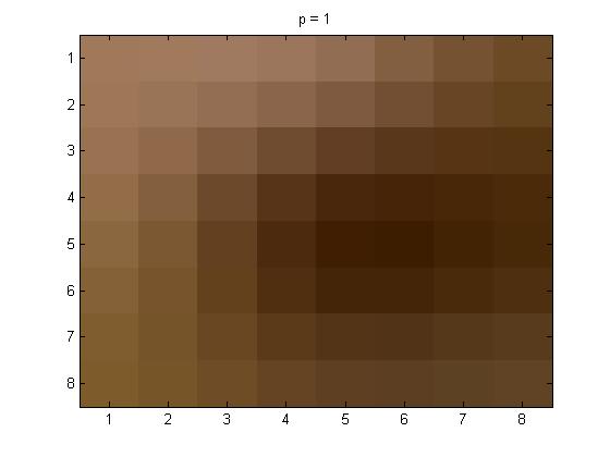
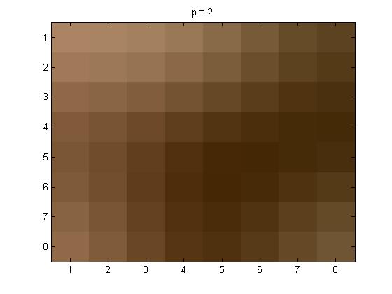
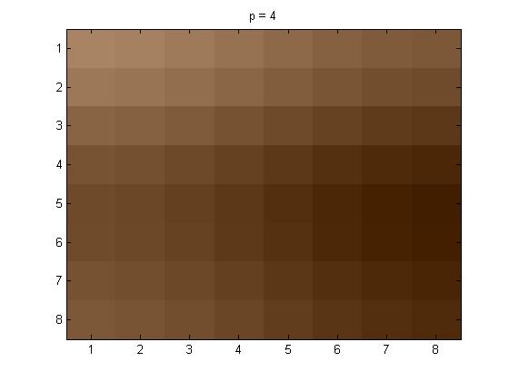
The Yq values are not included this time because there would be a matrix for each of the colors separately.
In this part of the project I used project5number5e.m, for the full picture, and I used p = 1, 2, 4, and 100 below are the pictures respectively:
But first as a reminder, here is the original photo in color:
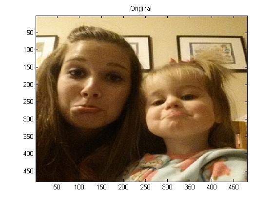


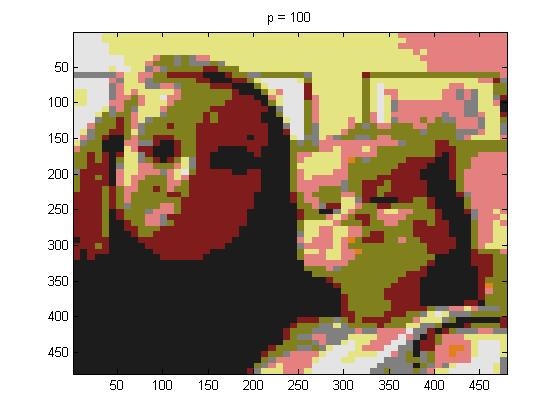
It can be seen that p = 1 practically looks identical to the original picture. But as p is increased the quality of the compressed image compared to the original is not nearly as good.
In this part of the project I was to obtain a color image, and transform the RGB values to luminance/color difference coordinates. Carry out the steps of Computer Problem 3 for Y, U, V separately by using JPEG quantization, and recombine as a color image.
In this part of the project, for the 8 \(\times\)8 I used project5number5ad.m. The pictures below are as follows: line (1): original grayscale, line (2): p = 1, p = 2, and p = 4.
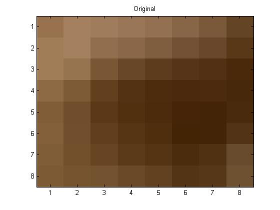
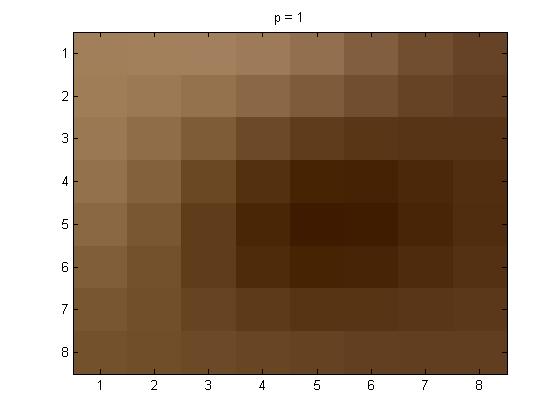
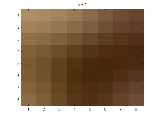
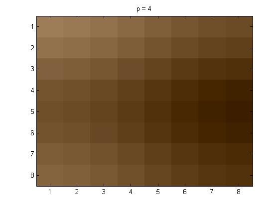
The Yq values are not included this time because there would be a matrix for each of the colors separately.
In this part of the project I used project5number5e.m, for the full picture, and I used p = 1, 2, 4, and 100 below are the pictures respectively:
But first as a reminder, here is the original photo in color:

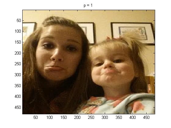


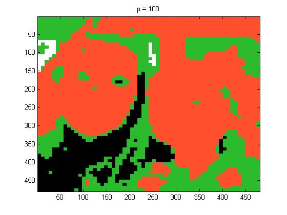
The last image is unrecognizable, I would think it was something for Christmas with how the colors got grouped.
Overall I thought this was a really fun project, because I like pictures. But I think that it is clear from my project that as we increase p the quality of the compressed image decreases. Some other things that I can conclude is that if you do not remember to include multiplying p in your quantizing matrix, then nothing changes as you increase p. Also, I thought it was cool to learn that there are toolboxes that MATLAB. I was stuck for a while not knowing that dct( ) was already in MATLAB. Also something that I learned was that idct( ) is a function that is already defined in MATLAB.