Topography
Sea Surface Height
Sea Surface Temperature
Surface Wind Field
Below are links to PDF files containing projections of various Earth properties which can be used to create OctaGlobes.
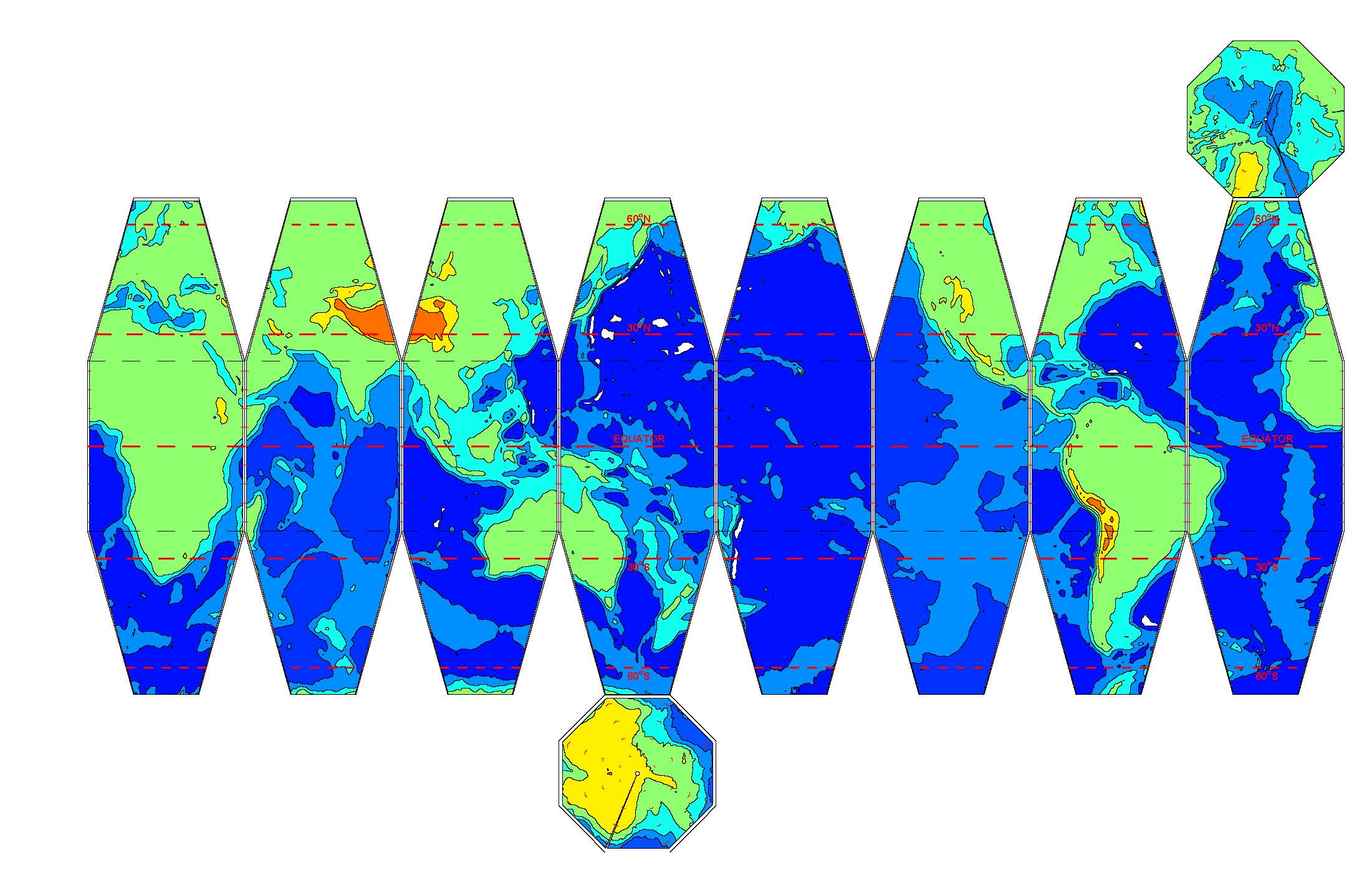
Construction tips: Card stock is best to create durable OctaGlobes but paper works also. The image above of 1 degree-resolution topography shows a typical OctaGlobe projection. To create OctaGlobe, cut out the entire complex shape, and fold along the boundary of each longitude section. Fold each sector at the latitude line separating the rectangle representing the tropics and the trapezoids representing mid-latitudes. Hold neighboring trapezoids so that their edges line up with each other, and tape together. At first the resulting shape may not seem too promising for representing a sphere, but towards the end it will automatically settle into the right shape. Fold and tape polar octagons to complete OctaSphere.
Some examples contain 1-page and 2-page projections in order to make a smaller or larger OctaGlobe. I hope to include additional fields in the near future. Donations (of fields) are welcome!
Height above sea level of solid Earth surface (land, ice, sea floor) from NOAA ETOPO5 data set. Original data is 1/12 degree resolution; maps are constructed by averaging neighboring grid points to 1/2 degree resolution (and further smoothing for One-Page map).
While topographic globes are commonly available, they often do not clearly show the large-scale height of the topography. The maps shown here show some interesting features such as the fact that almost all of Africa is more than 250 m above sea level, the Himalayas and Andes are significantly higher than the Rockies and Alps, and much of the Arctic consists of shallow continental shelf.
Projections: One-Page and Two Page (Page 1 and Page 2).Sea surface height relative to the geoid from satellite data. The geoid is what sea level would be if there were no forces on the ocean surface besides the Earth's gravity and centrifugal force). Data is on a 1/4 degree grid averaged over 2004-2008, and omits ice-covered regions near the poles. Shading shows speed based on geostrophic surface velocity.
Contours of constant sea surface height represent the flow paths of geostrophic surface velocity and sea surface slope is related to the geostrophic surface speed. Away from the equator, geostrophic flow represents most of the ocean flow for time-averaging much longer than a day. Thus sea surface height reveals the gyres and boundary currents of the global surface circulation.
Projections: One-Page and Two Page (Page 1 and Page 2).Sea surface temperature (SST) data from satellite infrared observations compiled at NOAA AVHRR version 2. Data is optimum interpolation to .25 degree resolution grid.
This field represents temperature on a single day (15 December 2005). For many purposes a climatological field showing averages over several years gives a more representative picture. Besides the general trend of SST getting colder near the poles and warmer near the tropics, some interesting features include the "Cold Tongue" of relatively cool water along the equator in the eastern Pacific, cool regions on the eastern edges of many basins, and warm tongues stretching poleward in the region of the Gulf Stream (western North Atlantic) and the Agulhas (western South Indian). A snapshot of SST looks similar to the seasonal climatology but also shows roughly 100 km wide features associated with mesoscale eddies and larger features associated with Tropical Instability Waves at the edge of the Cold Tongue.
Projections: (Page 1 and Page 2).Wind velocity is taken from ERA interim reanalysis 2009-2012 average. Wind values are originally on constant pressure levels. For graphs these are interpolated to the estimated lowest level above topography, which uses lower pressure levels over mountains and polar ice caps. Concerning how representative a 4 year average is, I compared to a 2 year average (2008-2009) and found differences to be too small to make a noticible difference in an arrow plot such as this.
Projections: (Page 1 and Page 2). Posted: 26 August 2012
Last modified: 19 May 2016