<- Back to home

Project 1


Introduction

The stewart platform is a three dimensional platform with 6 degrees of freedom, or rather 6 strut lengths which control the orientations of the platform. In this project, we explore a two-dimensional analog: a triangular platform controlled by 3 struts, which are anchored to three points (\(0,0), (x_1,0)\), and (\(x_2,y_2)\)
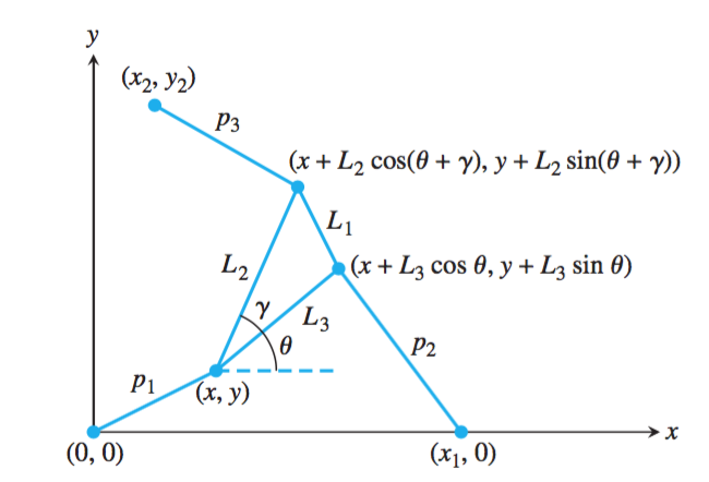
In this project, we examined the geometry of the 2D Stewart Platform in order to solve its forward kinematics, or rather the orientation of our platform given the individual strut lengths, and \(\gamma\). Our Matlab code creates a function in terms of a single variable \(\theta\), whose zeros correspond to different orientaions of the triangle.

From simple trigonometry, we obtain that $$ p_1^2 = x^2 + y^2 $$ $$p_2^2 = (x+ A_2)^2 + (y+ B_2)^2$$ $$ p_3^2 = (x+A_3)^2 + (y+B_3)^2$$

where

$$A_2 = L_3cos(\theta) - x_1 $$ $$B_2 = L_3sin(\theta)$$ $$A_3 = L_2cos(\theta + \gamma) - x_2 $$ $$B_3 = L_2sin(\theta +\gamma) - y_2$$

These equations provide a solution to the inverse kinematics problem. Given an angle \(\theta\), and position \((x,y)\), we can calculate the corresponding strut lengths for the platform. The forward kinematics problem, however, is more complex

We can solve the forward kinematics by eliminating \(x\) and \(y\).

We set $$ x = \frac{N_1}{D} = \frac{B_3(p_2^2 - p_1^2 - A_)2^2 - B_2^2) - B_2(p_3^2 - p_1^2 - A_3^2 - B_3^2)}{2(A_2B_3 - B_2A_3)}$$ $$ y = \frac{N_2}{D} = \frac{-A_3(p_2^2 - p_1^2 - A_2^2 - B_2^2) + A_2(p_3^2 - p_1^2 - A_3^2 - B_3^2)}{2(A_2B_3 - B_2A_3)}$$

Substituting back into the first equation, we get a single equation in the variable \(\theta\), $$f = N_1^2 + N_2^2 - p_1^2D^2 = 0. $$
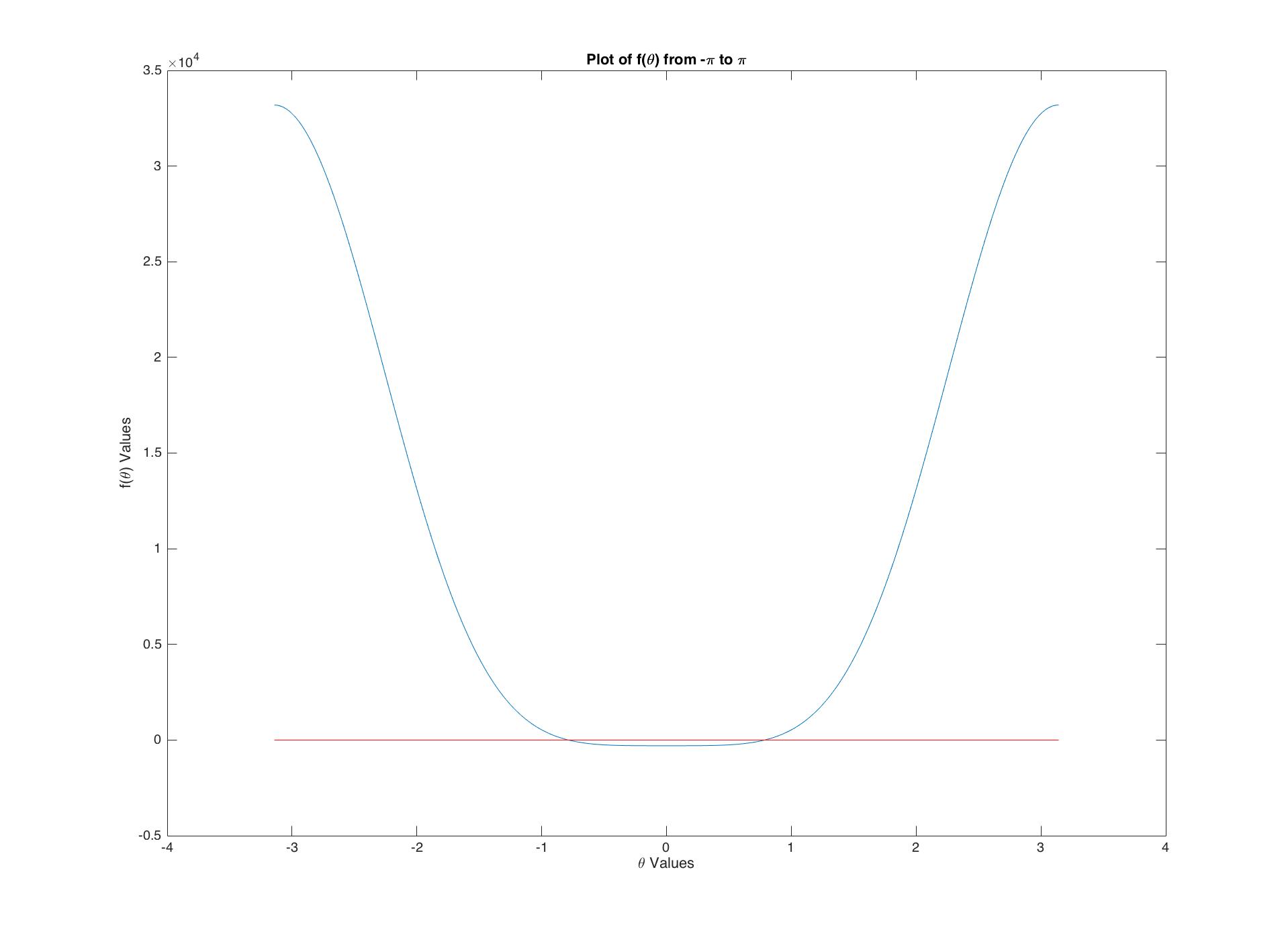
Part II: Graph of \(f(\theta)\)

Our Matlab code creates the function described in the introduction for a given set of parameters. We began by plotting \(f(\theta)\) for a given set of sample values of parameters in order to test our function \(L_1,L_2, L_3, p_1, p_2,p_3, \gamma\), with a set of anchoring points \(\{(0,0), (4,0),(0,4)\}\).


The parameter test values were as follows: \(L_1 = 2\) \(L_2 = L_3 = \sqrt2\)
\(p_1 = p_2 = p_3 = \sqrt2\)
\(\gamma = \frac{\pi}{2}\)

This function's zeros for the given parameters are truly at \(\frac{\pi}{4}\) and \(\frac{-\pi}{4}\). Upon calculating \(f(\theta)\) for these values we obtain the same backward error of \(-2.273 * 10^{-13}\). This is small enough a value to accept these values as the true zeros.


Part III

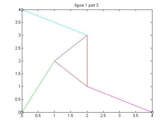
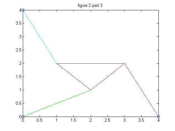
The graph in the previous section had two zeroes, each of which corresponds to a pose in the two-dimensional Stewart Platform. The pose corresponding to the root \(\theta = \frac{\pi}{4}\) returned, as expected, a coordinate of \((x,y) = (2,1)\) while \(\theta = -\frac{\pi}{4}\) returned \((x,y) = (1,2)\). The plots of each orientations were obtained by manually plotting the vectors in Matlab after solving for \(\theta\) These plots are shown below:


Part IV

We now construct poses for the Stewart Platform specified by \(x_1 = 5\), \((x_2,y_2) = (0,6)\), \(L_1 = L_3 = 3\), \(L_2 = 3\sqrt{2}\), \(\gamma = \frac{\pi}{4}\), \(p_1 = p_2 =5\), and \(p = 3\).

\(\theta\) \(X\) \(Y\) Plot
2.1159 4.5718 2.0244
-0.7208 -1.3784 4.8063
-0.3310 -0.9147 4.9156
1.1437 4.4818 2.2167


Part V

We repeat the process in part 4 but we must change the second strut length, p2, so that we wind up with 6 poses instead of 4. We chose p2 = 7.005 for our new strut length, and then followed through with the problem as before.

Theta X Y Plot
-0.6587 -4.3488 2.4673
-0.3813 -4.7809 1.4637
0.0481 -4.9488 0.7134
0.4603 -0.8223 4.9319
0.9775 2.2955 4.4419
2.5144 3.2114 3.8324


Part VI

Once more we repeat the process in part 4 and part 5 but this time we look for parameters that gives us only 2 roots and 2 poses. To accomplsih this we used P2 = 9 for our flexible strut and that produced two poses.

Theta X Y Plot
1.5479 0.7100 4.9493
2.2989 1.3916 4.8024