Project 5: Audio Compression
Aidan Curran
Contents
Background
Reality Check 11 Chapter 11 Numerical Analysis Problems 1-5
List of Code used
Initial Code from textbook: Simple Audio Codec
Code for part 1: Audio Compression Adapted from Simple Codec
Code for part 2: Audio Compression for chords
Code for part 2: Compression Portion for chords
Code for part 3: Compression using a windowing function
Code for part 3: Compression for chords w/ a windowing function
Code for part 3: Compression Portion for chords 2
Code for part 5: Audio Compression for incoming audio files
Problem 1
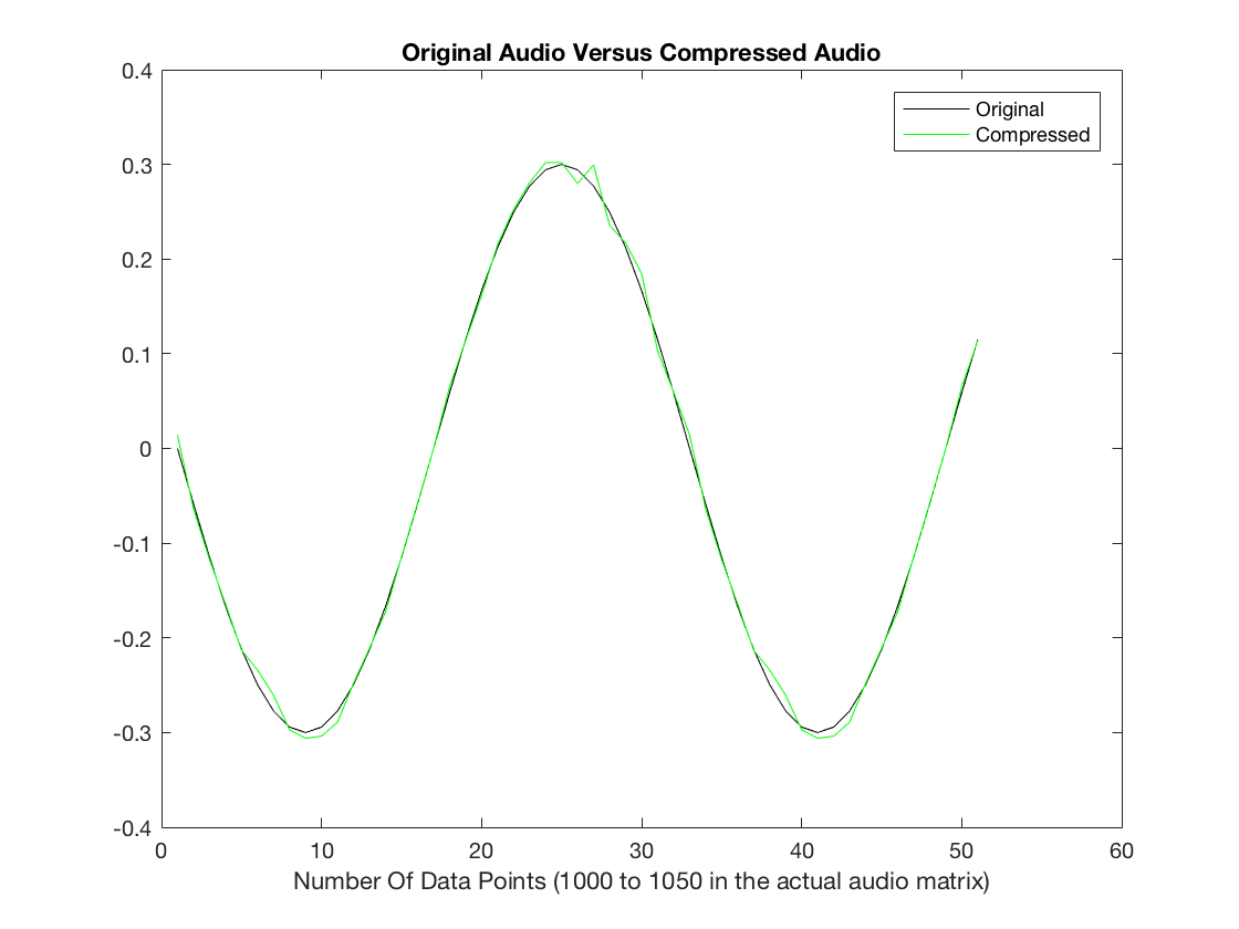
Investigate the ability of MDCT to represent puretones. Begin with  bits per window of size
  . Pick a tone of frequency between 100 Hz and 1000 Hz, and calculate the difference (as RMSE) between the original signal and the signal after encoding/decoding. You should cut the original signal to
  for comparison with the output signal, since the latter lacks n entries at the left and right ends. Plot a short section of the original and decoded signal.
Here is the code used for this part: Audio Comp 1
The frequency I picked for this part is 256 Hz
out=audioComp1(cos((1:2^(12))*2*pi*(FREQUENCY)/2^(13)));
out=audioComp1(cos((1:2^(12))*2*pi*256/2^(13)));
RMSE =
    0.0091
Initial Audio
Compressed Audio
Problem 2
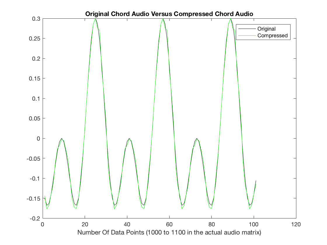
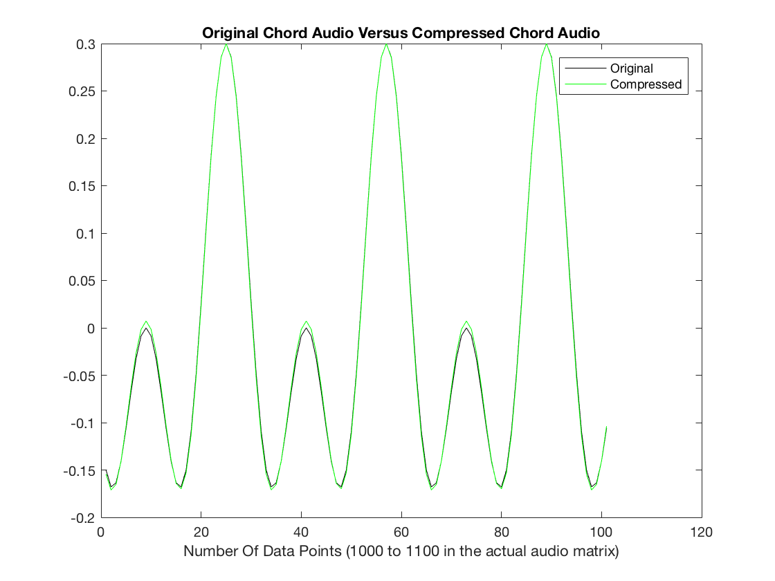
Build chords and evaluate the RMSE as in Step 1. Simple intervals can be constructed by a simple addition of multiple pure tones. Rational ratios of frequencies with low numerators and denominators are pleasing to the ear: A 2 : 1 ratio of frequencies gives an octave, 1.25 : 1 ratio gives a third, a 1.5 : 1 gives a fifth, and so forth. How does the RMSE depend on the number of bits used in the coder?
Here is the code used for this part: Chords
Here is the code used for this part: Audio Comp 2
chords(256,2,1)
RMSE =
    0.0092
Initial Audio
Compressed Audio
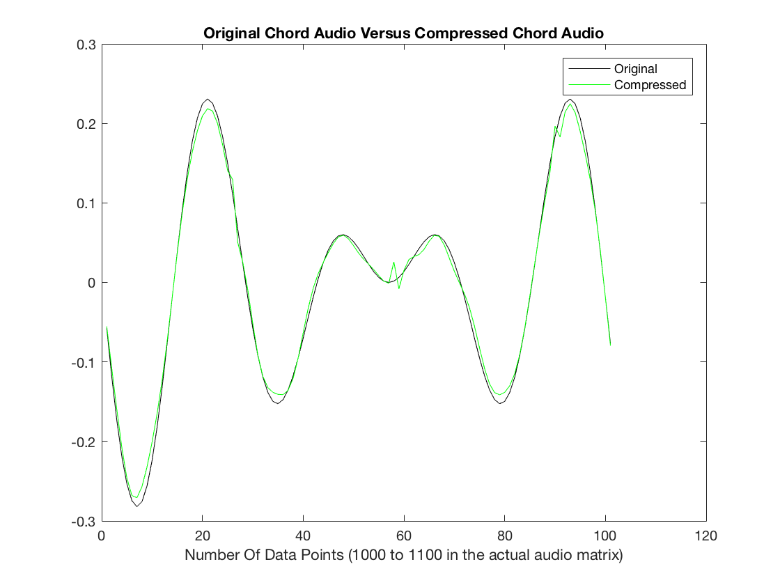
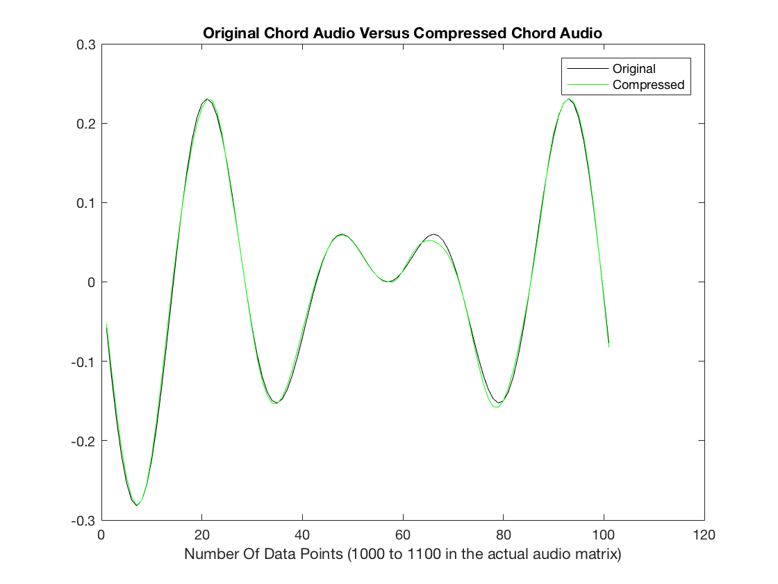
chords(256,1.25,1)
RMSE =
    0.0109
Initial Audio
Compressed Audio
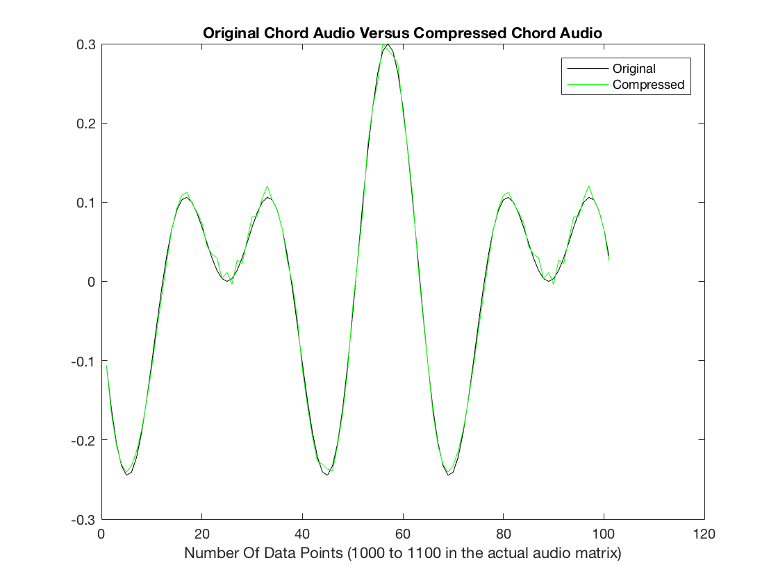
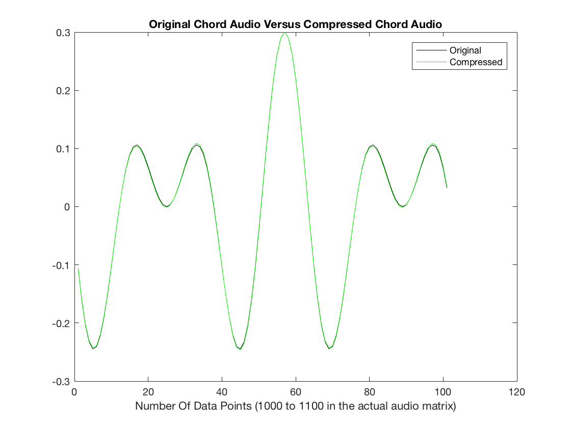
chords(256,1.5,1)
RMSE =
    0.0069
Initial Audio
Compressed Audio
     With a higher bit quantization, the RMSE is gets smaller and smaller.
     It also decreases the number of higher and lower frequency bits being
     removed or adjusted.
Problem 3
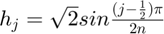
A "windowing function" is often used to reduce codec error, due to the fact that the function being represented is not periodic over the window, but is being represented by periodic functions. The windowing function scales the input signal  smoothly to zero at each end of the window, partially mitigating this problem. A common choice is to replace
  with
with  , where
  for a length 2n window, where
 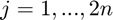 . To undo the windowing function, multiply the inverse MDCT output
  componentwise by the same
  . This results in multiplying
  componentwise by the second half of the
  , and
, and  by the first half
  before combining into the decoded signal. Compare RMSE, plots, and audible sound as in Steps 1 and 2.
Here is the code used for this part: Audio Comp 3
Here is the code used for this part: Chords 2
Here is the code used for this part: Audio Comp 4
out=audioComp3(cos((1:2^(12))*2*pi*256/2^(13)));
RMSE =
    0.0011
Initial Audio
Compressed Audio
chords2(256,2,1)
RMSE =
    0.0037
Initial Audio
Compressed Audio
chords2(256,1.25,1)
RMSE =
    0.0048
Initial Audio
Compressed Audio
chords2(256,1.5,1)
RMSE =
    0.0016
Initial Audio
Compressed Audio
Problem 4
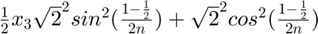
Explain the method for undoing the windowing that is suggested in Step 3. In other words, assume that if  and
and  are each multiplied componentwise by the entire windowing function
  , and
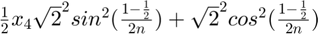
, and  and
and  in equation (11.38) are each multiplied
= [x1h1 ; x2h2 ; x3h3 ; x4h4]
= [x3h1 ; x4h2 ; x5h3 ; x6h4]
[x3; x4]= 1/2 ()n,...,2n-1 + 1/2 ()0,...,n-1
x_{3}
![$\frac{1}{2}x_{3}[h_{3}^2 + h_{1}^2]$](AudioCompression_eq15637746556180942652.png)

x_{4}
![$\frac{1}{2}x_{4}[h_{4}^2 + h_{1}^2]$](AudioCompression_eq12472934519018375565.png)

Problem 5
Import a .wav file with the MATLAB audioread command, or download an audio file of your choice. (Alternatively, load handel can be used. If you download a stereo file, you will need to work with each channel separately.) Reproduce the file (or a segment of it) using various values of b and with and without windowing. Compute RMSE for your choices of parameters and exhibit the results using the sound command.
Here is the code used for this part: Audio Comp 5
The song that I chose to demonstrate compression is the Tristram Theme from Diablo Soundtrack.
This is what the original song sounds like:
There are various examples of different quantization bit sizes with and without windowing. To start, I went with a low bit quantization.
Compressed Audio - b Value: 2 Windowing: No
audioComp5(2,0)
RMSE =
    0.0200
Compressed Audio - b Value: 2 Windowing: Yes
audioComp5(2,1)
RMSE =
    0.0175
Compressed Audio - b Value: 4 Windowing: No
audioComp5(4,0)
RMSE =
    0.0069
Compressed Audio - b Value: 4 Windowing: Yes
audioComp5(4,1)
RMSE =
    0.0049
Compressed Audio - b Value: 6 Windowing: No
audioComp5(6,0)
RMSE =
    0.0019
Compressed Audio - b Value: 6 Windowing: Yes
audioComp5(6,1)
RMSE =
    0.0014
Compressed Audio - b Value: 8 Windowing: No
audioComp5(8,0)
RMSE =
   4.8007e-04
Compressed Audio - b Value: 8 Windowing: Yes
audioComp5(8,1)
RMSE =
   4.0253e-04